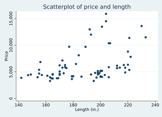
graphtwowayscatter price length, title("Scatterplot of price and length")
scatter price length, title("Scatterplot of price and length")
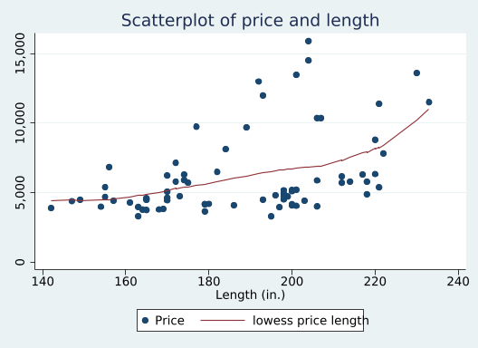
40.1.2.2 Adding a Lowess Smoother
Adding the lowess’ smoother is easy as well. To do this we are going to append two graph twoway plots. Specifically, we are going to append scatter and lowess. We append two plots by using double-pipes — ||.
graphtwowayscatter price length || lowess price length, title("Scatterplot of price and length")
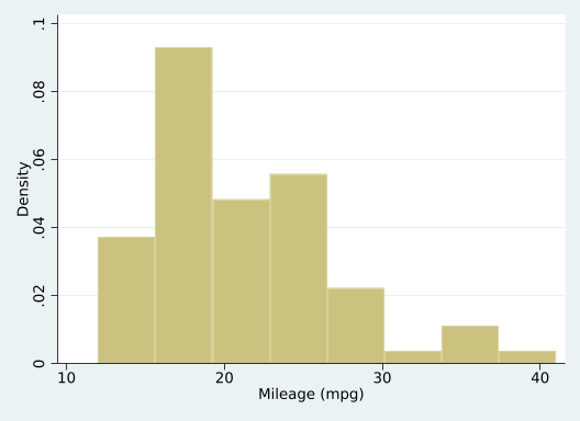
40.2 直方图
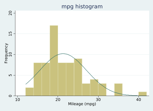
To create a histogram using commands, just type histogram followed by the variable name, e.g. histogram mpg, if you want to look at miles per gallon, you would type:
histogram mpg
(bin=8, start=12, width=3.625)
Often the default settings of the histogram may not be the best representation of your data. There are a number of useful options with the histogram command, including width with allows you to specify bin width, frequency which changes the y-axis to reflect frequency instead of density and normal which overlays a normal curve onto your graphic. You can also modify the title and axes of the graph using syntax options.
      Source |       SS           df       MS      Number of obs   =        74
-------------+----------------------------------   F(1, 72)        =     20.26
       Model |   139449474         1   139449474   Prob > F        =    0.0000
    Residual |   495615923        72  6883554.48   R-squared       =    0.2196
-------------+----------------------------------   Adj R-squared   =    0.2087
       Total |   635065396        73  8699525.97   Root MSE        =    2623.7

------------------------------------------------------------------------------
       price | Coefficient  Std. err.      t    P>|t|     [95% conf. interval]
-------------+----------------------------------------------------------------
         mpg |  -238.8943   53.07669    -4.50   0.000    -344.7008   -133.0879
       _cons |   11253.06   1170.813     9.61   0.000     8919.088    13587.03
------------------------------------------------------------------------------
To get standardized coefficients we add the beta option to our command.
regress price mpg, beta
      Source |       SS           df       MS      Number of obs   =        74
-------------+----------------------------------   F(1, 72)        =     20.26
       Model |   139449474         1   139449474   Prob > F        =    0.0000
    Residual |   495615923        72  6883554.48   R-squared       =    0.2196
-------------+----------------------------------   Adj R-squared   =    0.2087
       Total |   635065396        73  8699525.97   Root MSE        =    2623.7

------------------------------------------------------------------------------
       price | Coefficient  Std. err.      t    P>|t|                     Beta
-------------+----------------------------------------------------------------
         mpg |  -238.8943   53.07669    -4.50   0.000                -.4685967
       _cons |   11253.06   1170.813     9.61   0.000                        .
------------------------------------------------------------------------------
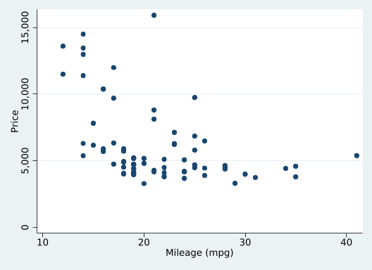
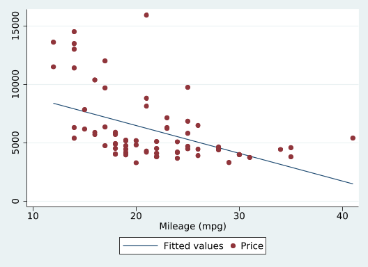
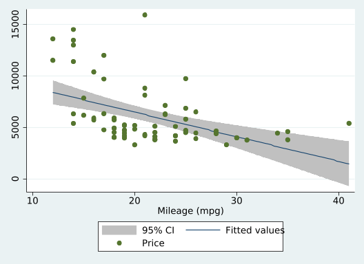
Visualizing Regression Lines
graphtwowayscatter price mpg
Add the regression line to the plot. The lfit graph command allows us to do this (lfit stands for linear fit). However, we don’t want the regression line in isolation. We want it on top of the scatterplot. Stata lets you combine twoway graphs in one of two ways: (1) using parentheses or (2) using pipes.