             species        temp            rate
 O. exclamationis:14   Min.   :17.20   Min.   : 44.30
 O. niveus       :17   1st Qu.:20.80   1st Qu.: 59.45
                       Median :24.00   Median : 76.20
                       Mean   :23.76   Mean   : 72.89
                       3rd Qu.:26.35   3rd Qu.: 85.25
                       Max.   :30.40   Max.   :101.70
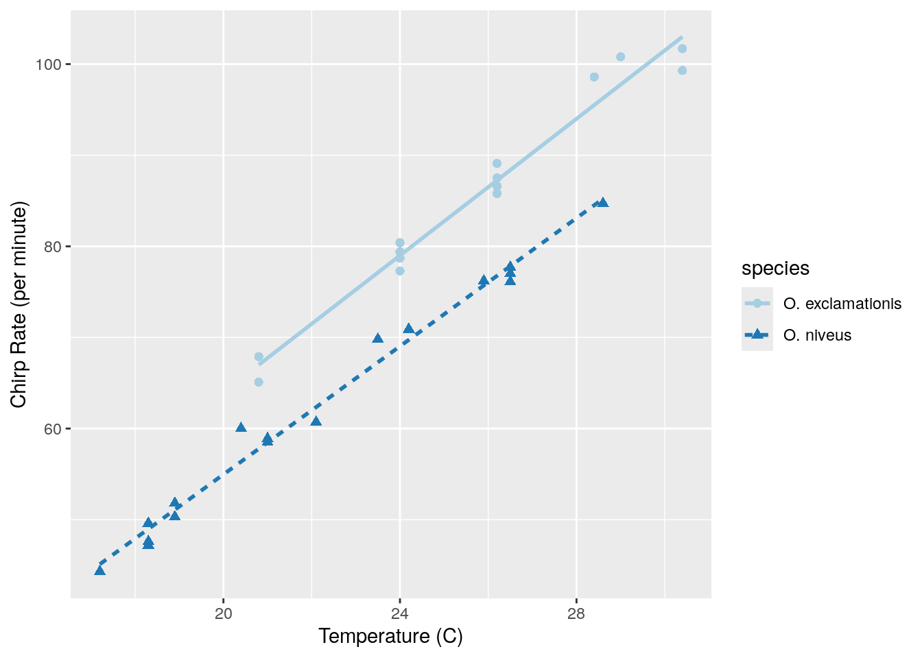
16.2 可视化两种物种温度与鸣叫频率的关系
# Plot the temperature on the x-axis, the chirp rate on the y-axis. The plot# elements will be colored differently for each species:ggplot(crickets, aes(x = temp, y = rate, color = species, 1pch = species,2lty = species )) +# Plot points for each data point and color by speciesgeom_point(size =2) +# Show a simple linear model fit created separately for each species:geom_smooth(method = lm, se =FALSE, alpha =0.5) +scale_color_brewer(palette ="Paired") +labs(x ="Temperature (C)", y ="Chirp Rate (per minute)")
1
pch = species : 这个参数指定了数据点的形状 (point character) 将根据 species 变量的不同取值而变化。每个不同的 species 可能对应不同的形状,这有助于在图中区分不同种类的数据点。
2
lty = species : 这个参数指定了线条的类型 (line type) 将根据 species 变量的不同取值而变化。每个不同的 species 可能对应不同的线条类型,这有助于在图中区分不同种类的线条。
16.3 交互作用的几种表达方法
result1 <- rate ~ temp + species + temp:species# A shortcut can be used to expand all interactions containing# interactions with two variables:result2 <- rate ~ (temp + species)^2# Another shortcut to expand factors to include all possible# interactions (equivalent for this example):result3 <- rate ~ temp * species
interaction_fit1 <-lm(rate ~ (temp + species)^2, data = crickets) # To print a short summary of the model:interaction_fit1
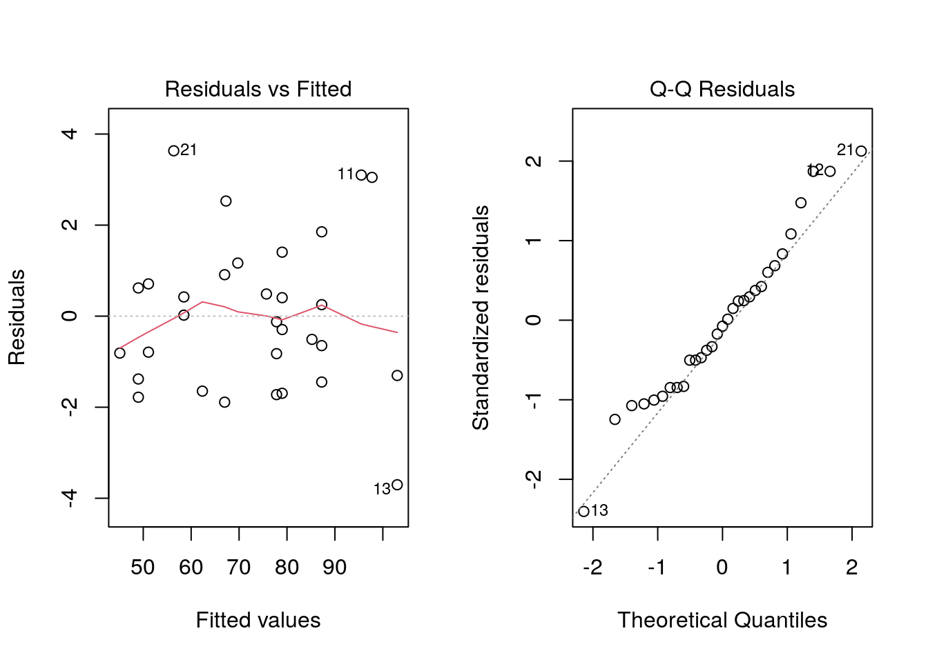
# Place two plots next to one another:par(mfrow =c(1, 2))# Show residuals vs predicted values:plot(interaction_fit3, which =1)# A normal quantile plot on the residuals:plot(interaction_fit3, which =2)
# Fit a reduced model:main_effect_fit <-lm(rate ~ temp + species, data = crickets) # Compare the two:anova(main_effect_fit, interaction_fit3)
Res.Df
RSS
Df
Sum of Sq
F
Pr(>F)
28
89.34987
NA
NA
NA
NA
27
85.07409
1
4.275779
1.357006
0.2542464
This statistical test generates a p-value of 0.25. This implies that there is a lack of evidence against the null hypothesis that the interaction term is not needed by the model.
We can use the summary() method to inspect the coefficients, standard errors, and p-values of each model term:
summary(main_effect_fit)
Call:
lm(formula = rate ~ temp + species, data = crickets)

Residuals:
    Min      1Q  Median      3Q     Max
-3.0128 -1.1296 -0.3912  0.9650  3.7800

Coefficients:
                  Estimate Std. Error t value Pr(>|t|)
(Intercept)       -7.21091    2.55094  -2.827  0.00858 **
temp               3.60275    0.09729  37.032  < 2e-16 ***
speciesO. niveus -10.06529    0.73526 -13.689 6.27e-14 ***
---
Signif. codes:  0 '***' 0.001 '**' 0.01 '*' 0.05 '.' 0.1 ' ' 1

Residual standard error: 1.786 on 28 degrees of freedom
Multiple R-squared:  0.9896,    Adjusted R-squared:  0.9888
F-statistic:  1331 on 2 and 28 DF,  p-value: < 2.2e-16