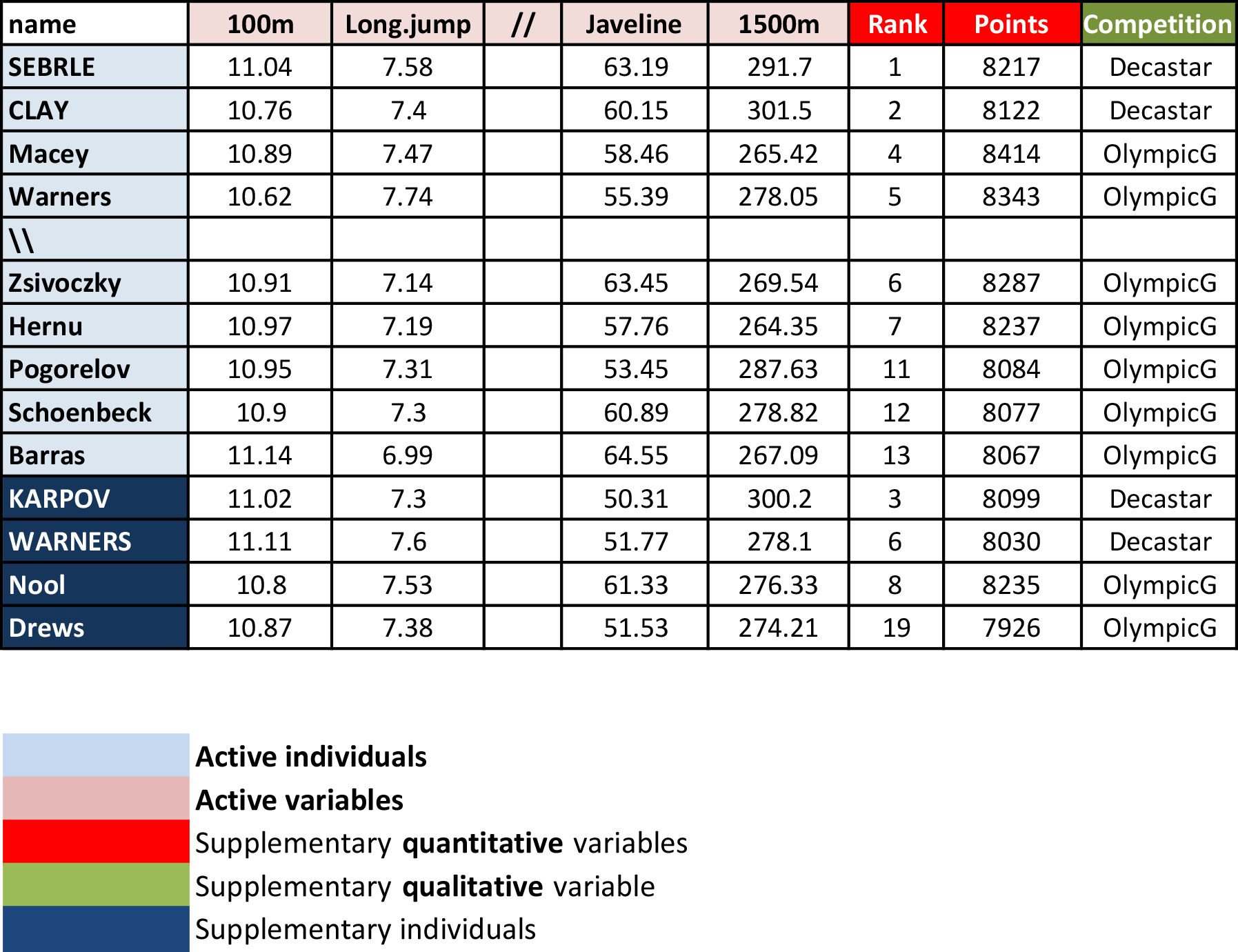
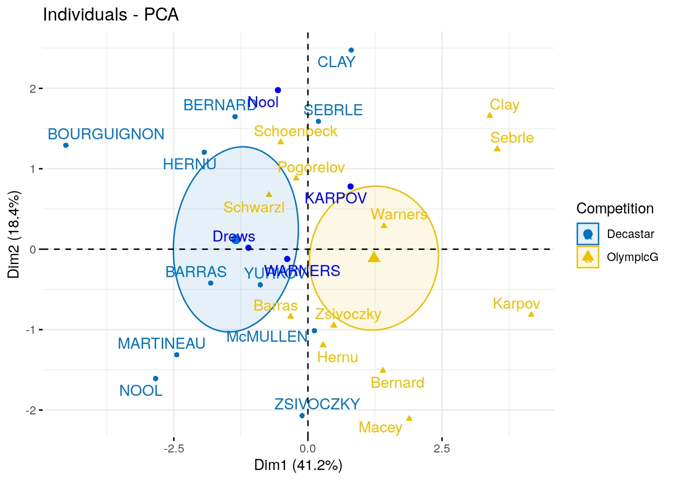
The data used here describes athletes’ performance during two sporting events (Desctar and OlympicG). It contains 27 individuals (athletes) described by 13 variables.
**Results for the Principal Component Analysis (PCA)**
The analysis was performed on 23 individuals, described by 10 variables
*The results are available in the following objects:
name description
1 "$eig" "eigenvalues"
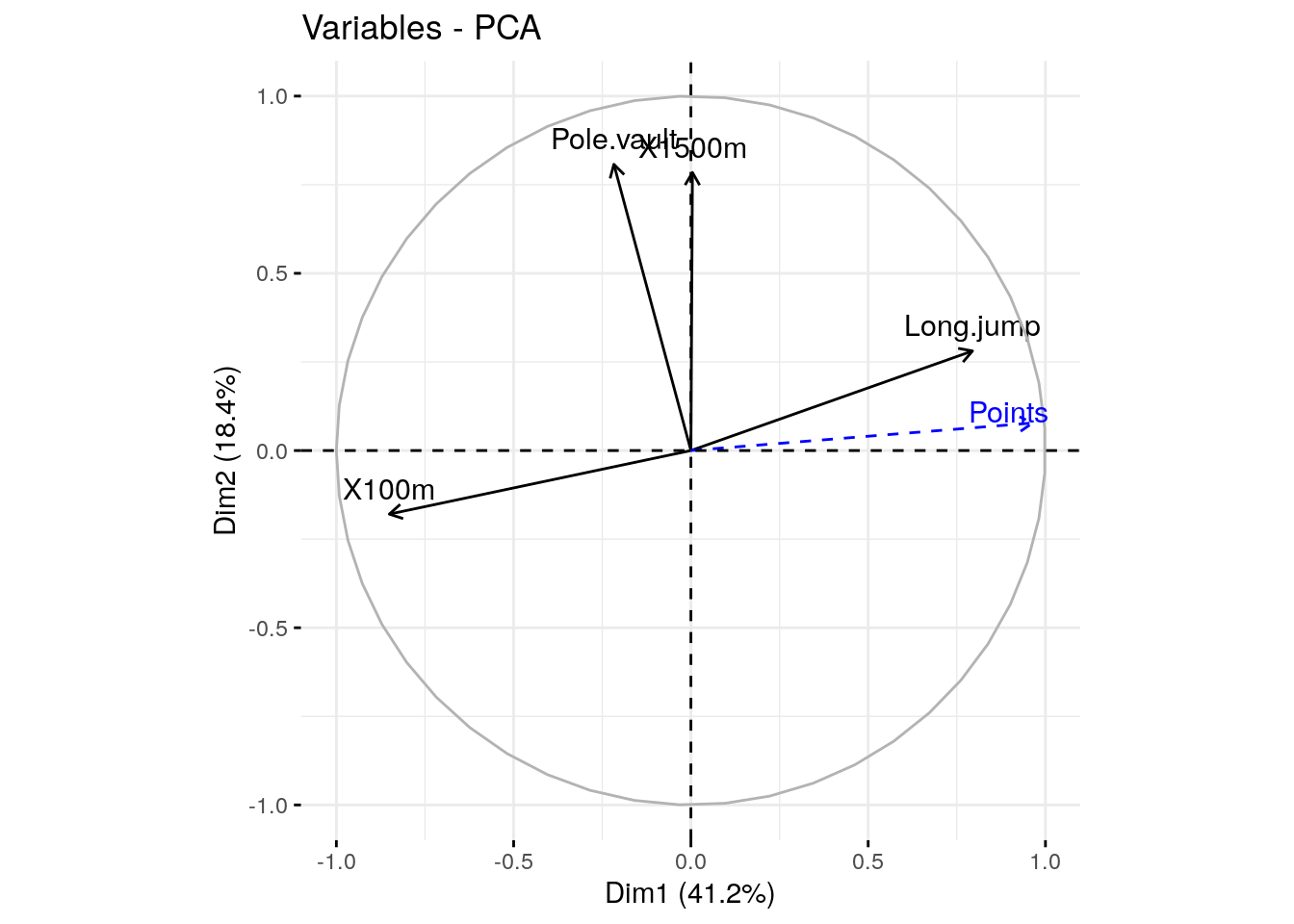
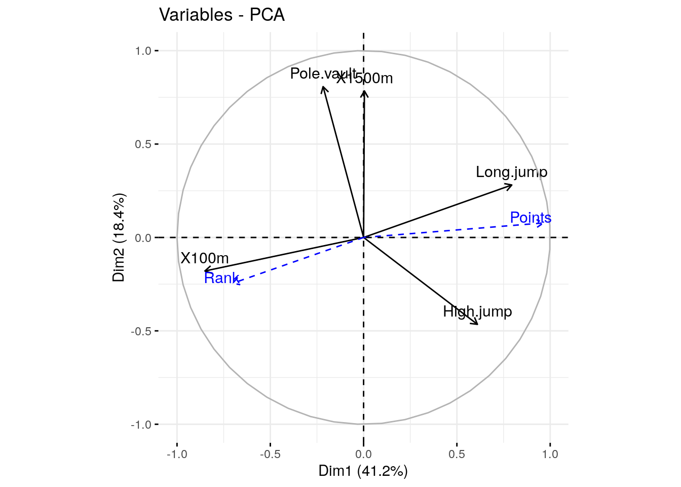
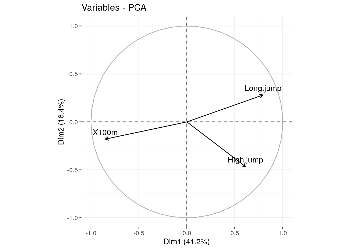
2 "$var" "results for the variables"
3 "$var$coord" "coord. for the variables"
4 "$var$cor" "correlations variables - dimensions"
5 "$var$cos2" "cos2 for the variables"
6 "$var$contrib" "contributions of the variables"
7 "$ind" "results for the individuals"
8 "$ind$coord" "coord. for the individuals"
9 "$ind$cos2" "cos2 for the individuals"
10 "$ind$contrib" "contributions of the individuals"
11 "$call" "summary statistics"
12 "$call$centre" "mean of the variables"
13 "$call$ecart.type" "standard error of the variables"
14 "$call$row.w" "weights for the individuals"
15 "$call$col.w" "weights for the variables"
Principal Component Analysis Results for variables
 ===================================================
  Name       Description
1 "$coord"   "Coordinates for the variables"
2 "$cor"     "Correlations between variables and dimensions"
3 "$cos2"    "Cos2 for the variables"
4 "$contrib" "contributions of the variables"
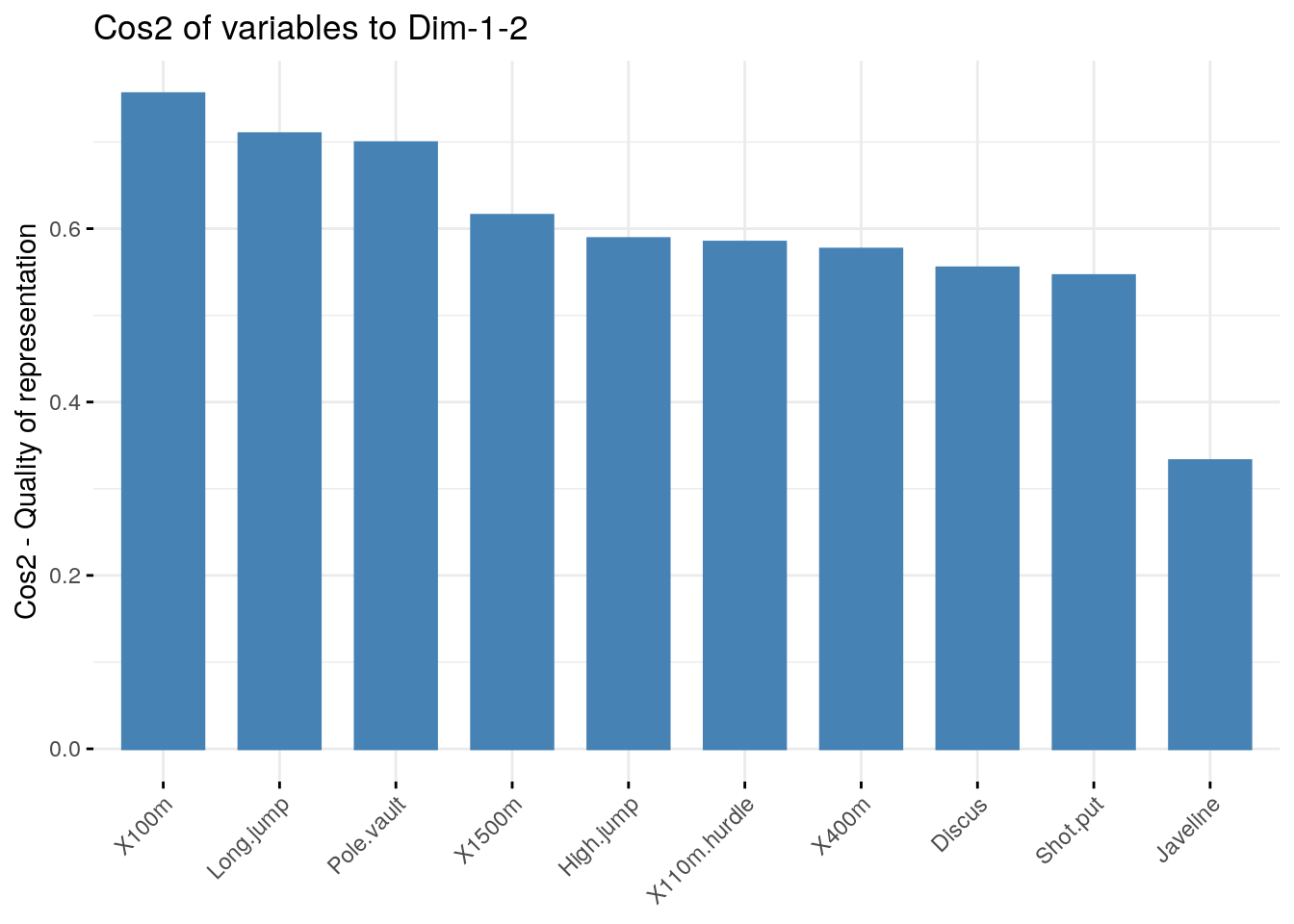
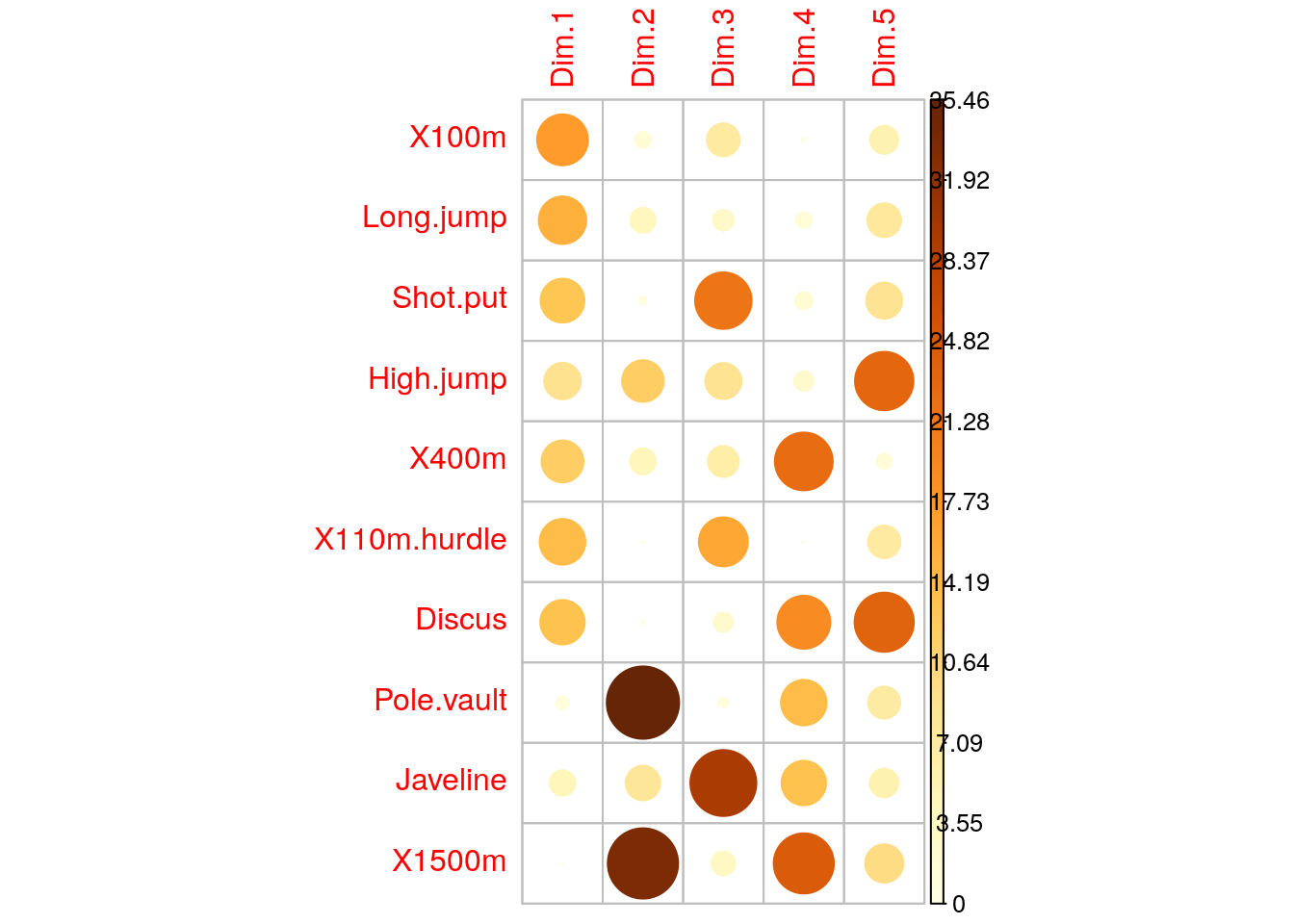
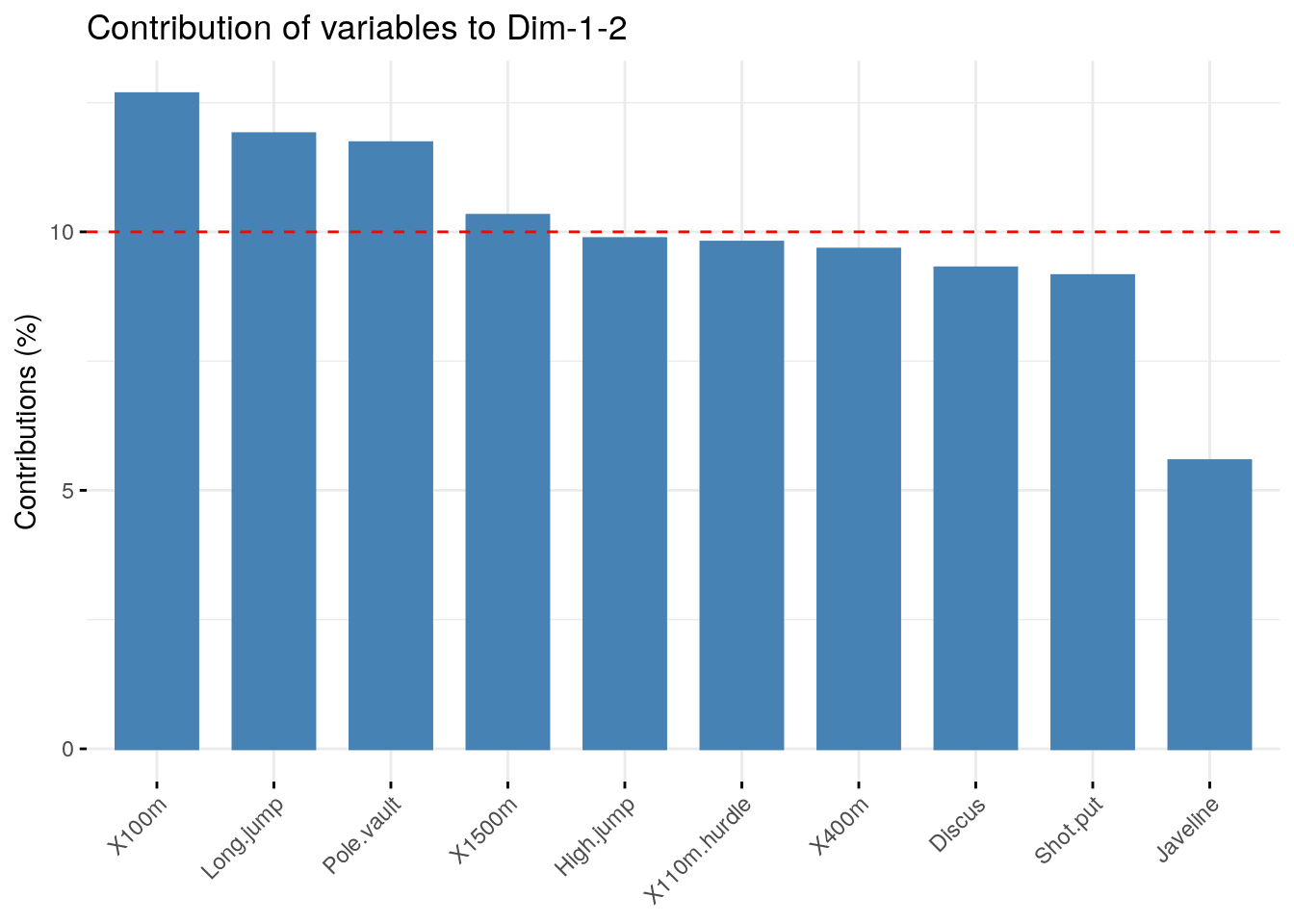
# Total cos2 of variables on Dim.1 and Dim.2fviz_cos2(res.pca, choice ="var", axes =1:2)
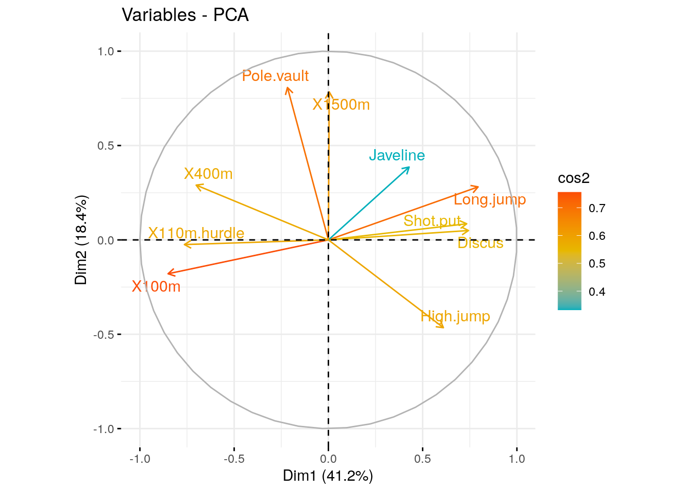
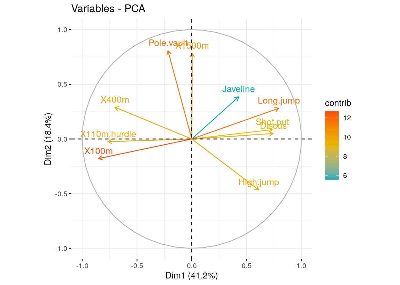
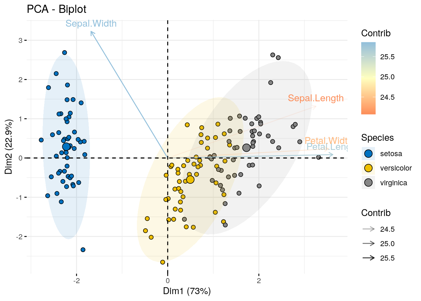
# Color by cos2 values: quality on the factor mapfviz_pca_var(res.pca, col.var ="cos2",gradient.cols =c("#00AFBB", "#E7B800", "#FC4E07"), repel =TRUE# Avoid text overlapping )
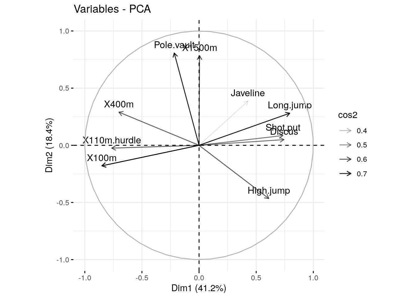
# Change the transparency by cos2 valuesfviz_pca_var(res.pca, alpha.var ="cos2")
# Change the transparency by contrib valuesfviz_pca_var(res.pca, alpha.var ="contrib")
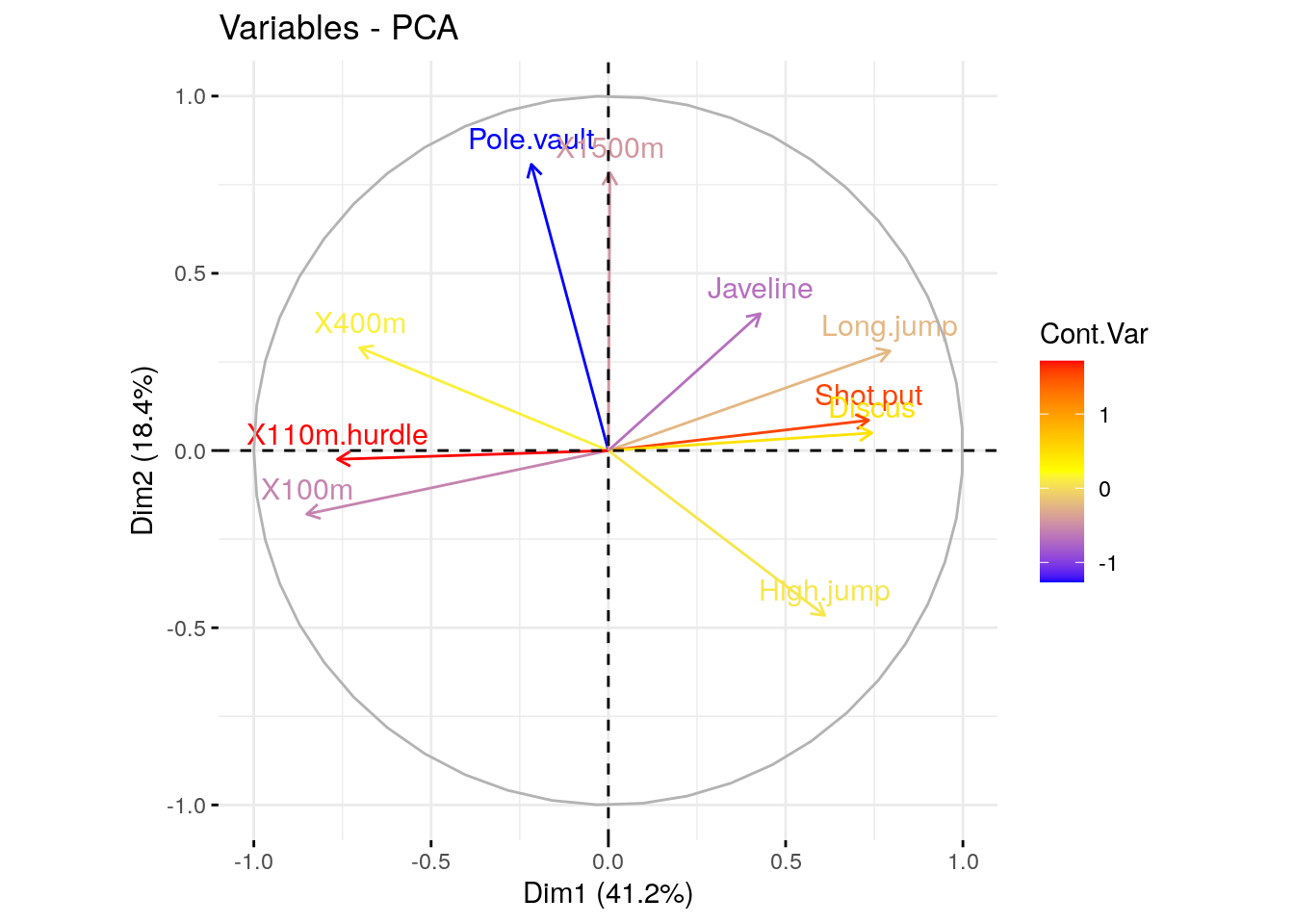
# Create a random continuous variable of length 10set.seed(123)my.cont.var <-rnorm(10)# Color variables by the continuous variablefviz_pca_var(res.pca, col.var = my.cont.var,gradient.cols =c("blue", "yellow", "red"),legend.title ="Cont.Var")
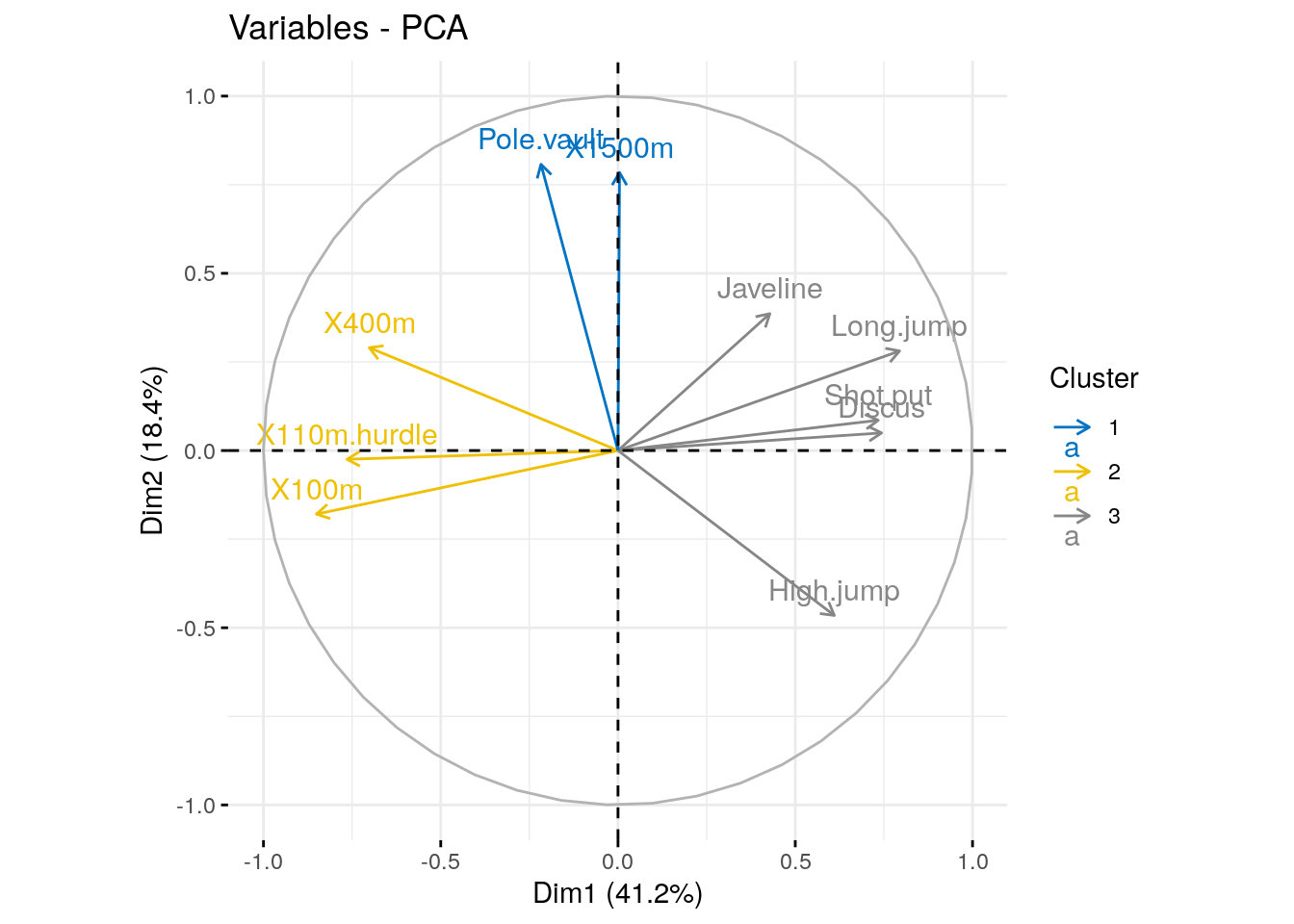
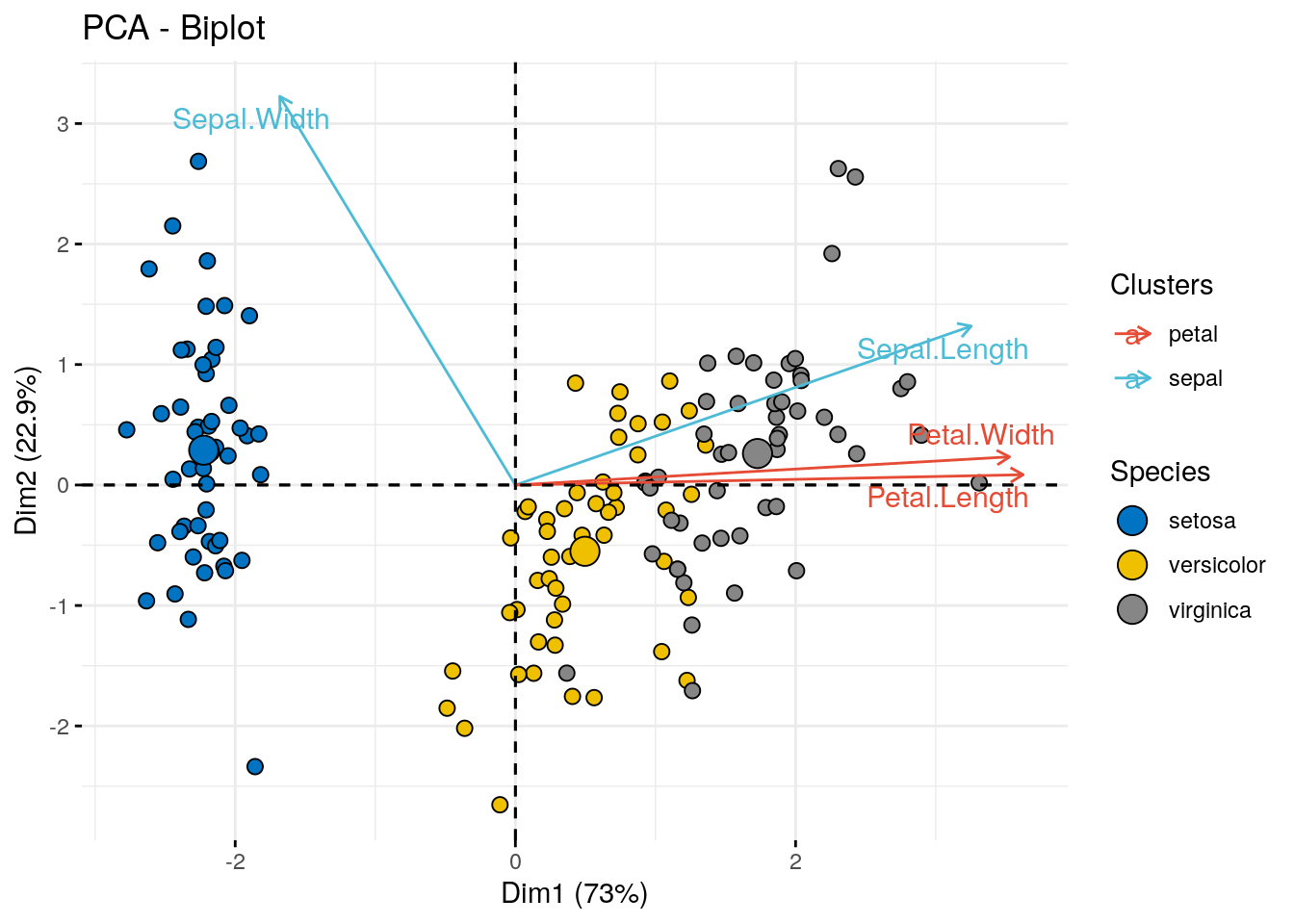
# Create a grouping variable using kmeans# Create 3 groups of variables (centers = 3)set.seed(123)res.km <-kmeans(var$coord, centers =3, nstart =25)grp <-as.factor(res.km$cluster)# Color variables by groupsfviz_pca_var(res.pca, col.var = grp, palette =c("#0073C2FF", "#EFC000FF", "#868686FF"),legend.title ="Cluster")
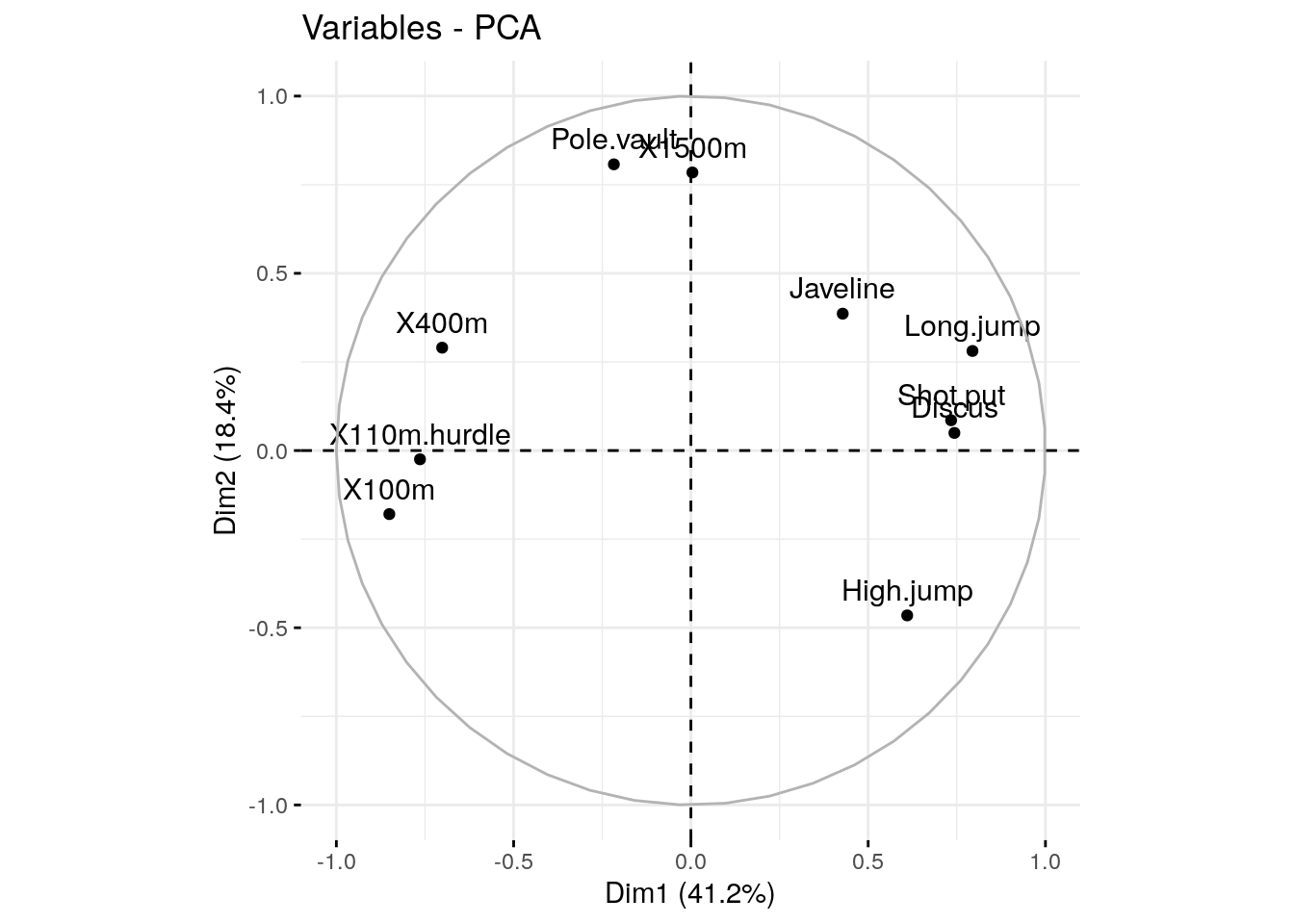
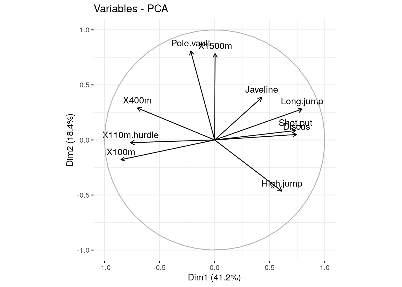
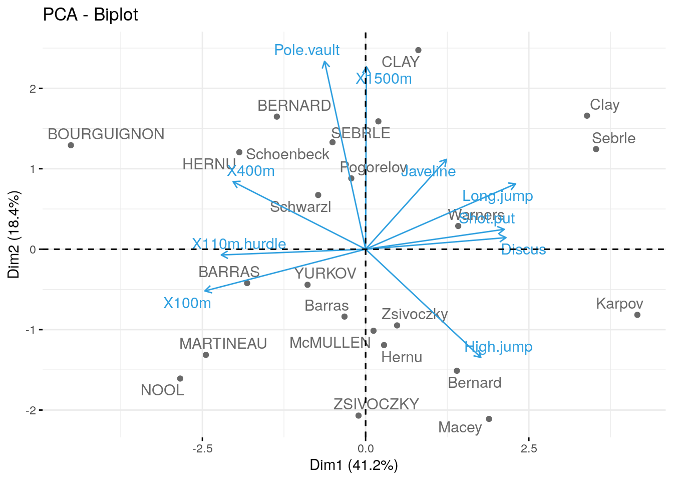
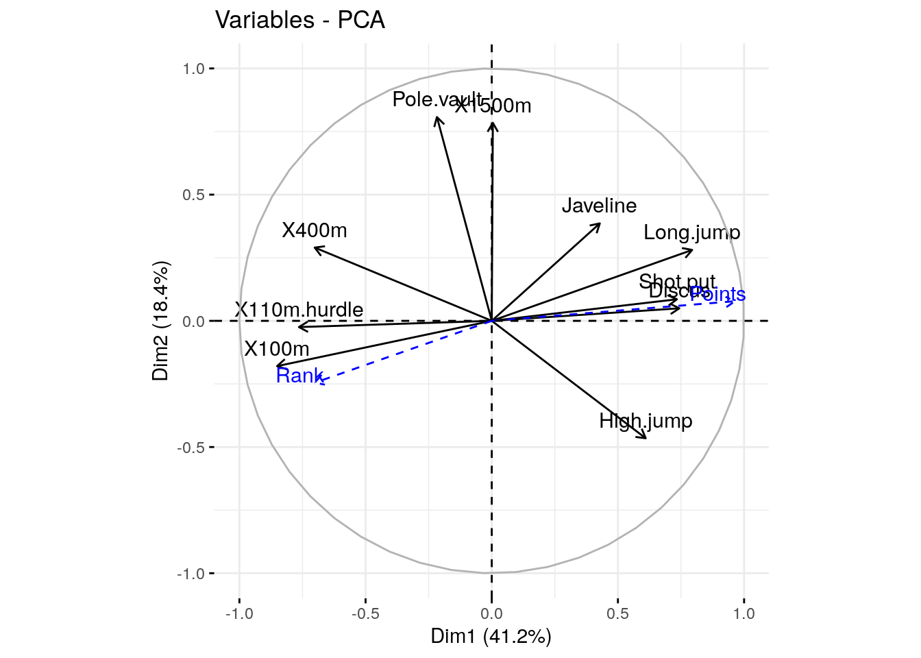
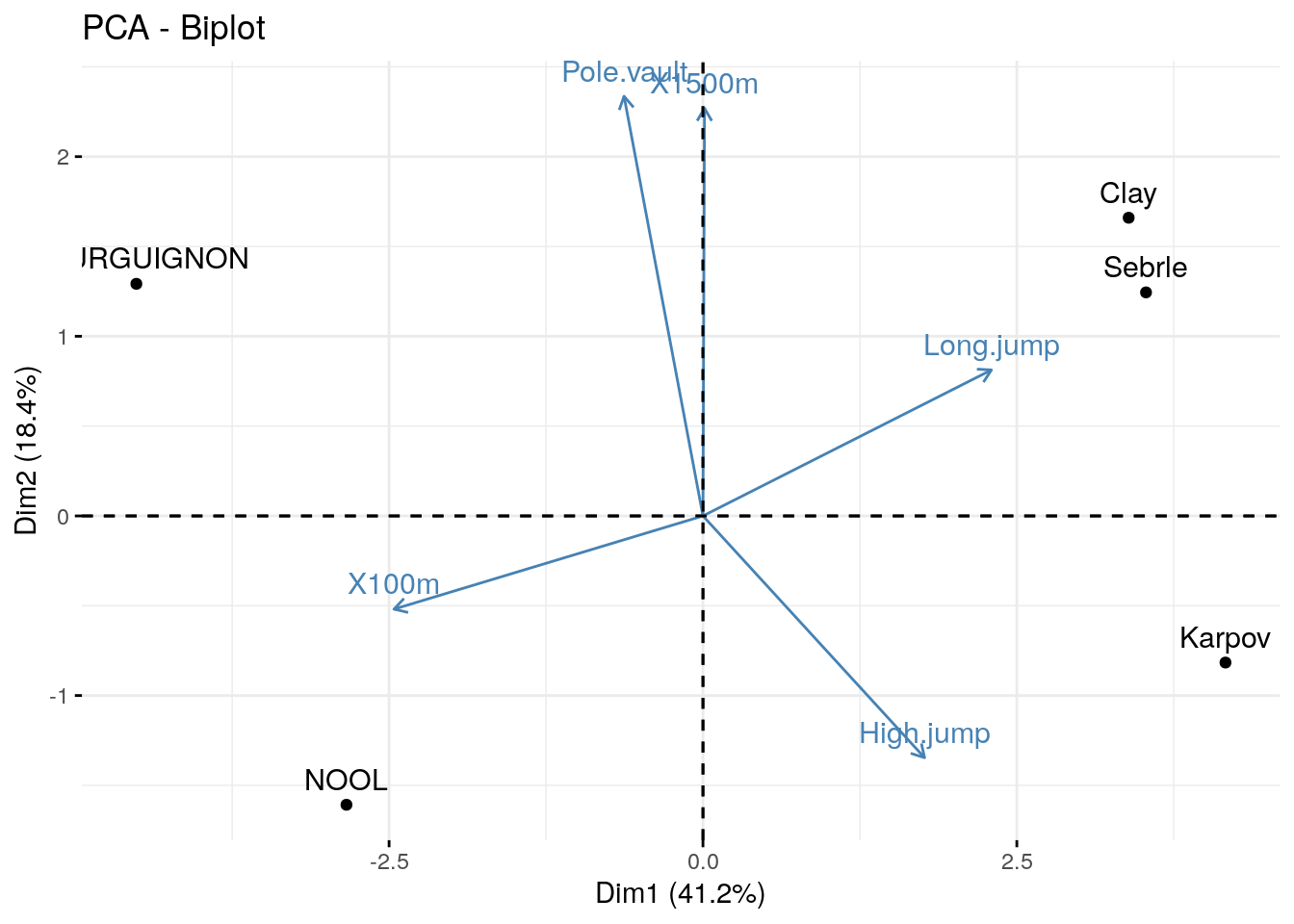
res.desc <-dimdesc(res.pca, axes =c(1,2), proba =0.05)# Description of dimension 1res.desc$Dim.1
Link between the variable and the continuous variables (R-square)
=================================================================================
             correlation      p.value
Long.jump      0.7941806 6.059893e-06
Discus         0.7432090 4.842563e-05
Shot.put       0.7339127 6.723102e-05
High.jump      0.6100840 1.993677e-03
Javeline       0.4282266 4.149192e-02
X400m         -0.7016034 1.910387e-04
X110m.hurdle  -0.7641252 2.195812e-05
X100m         -0.8506257 2.727129e-07
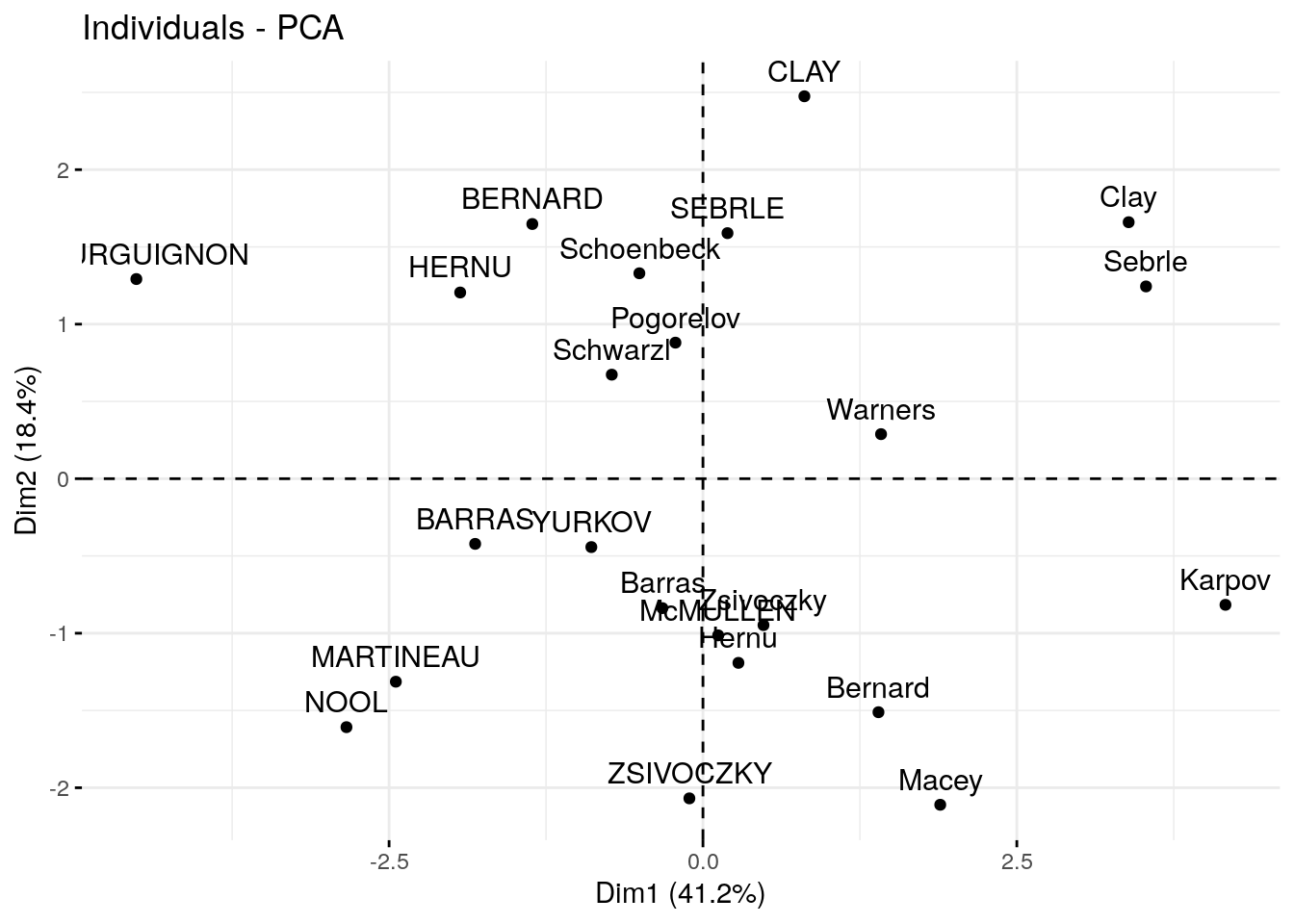
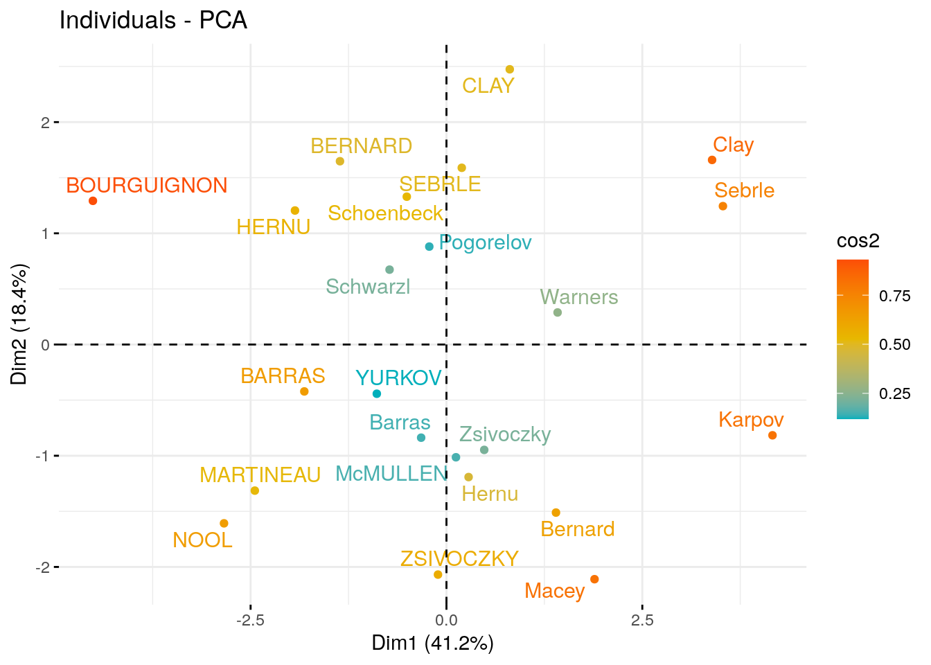
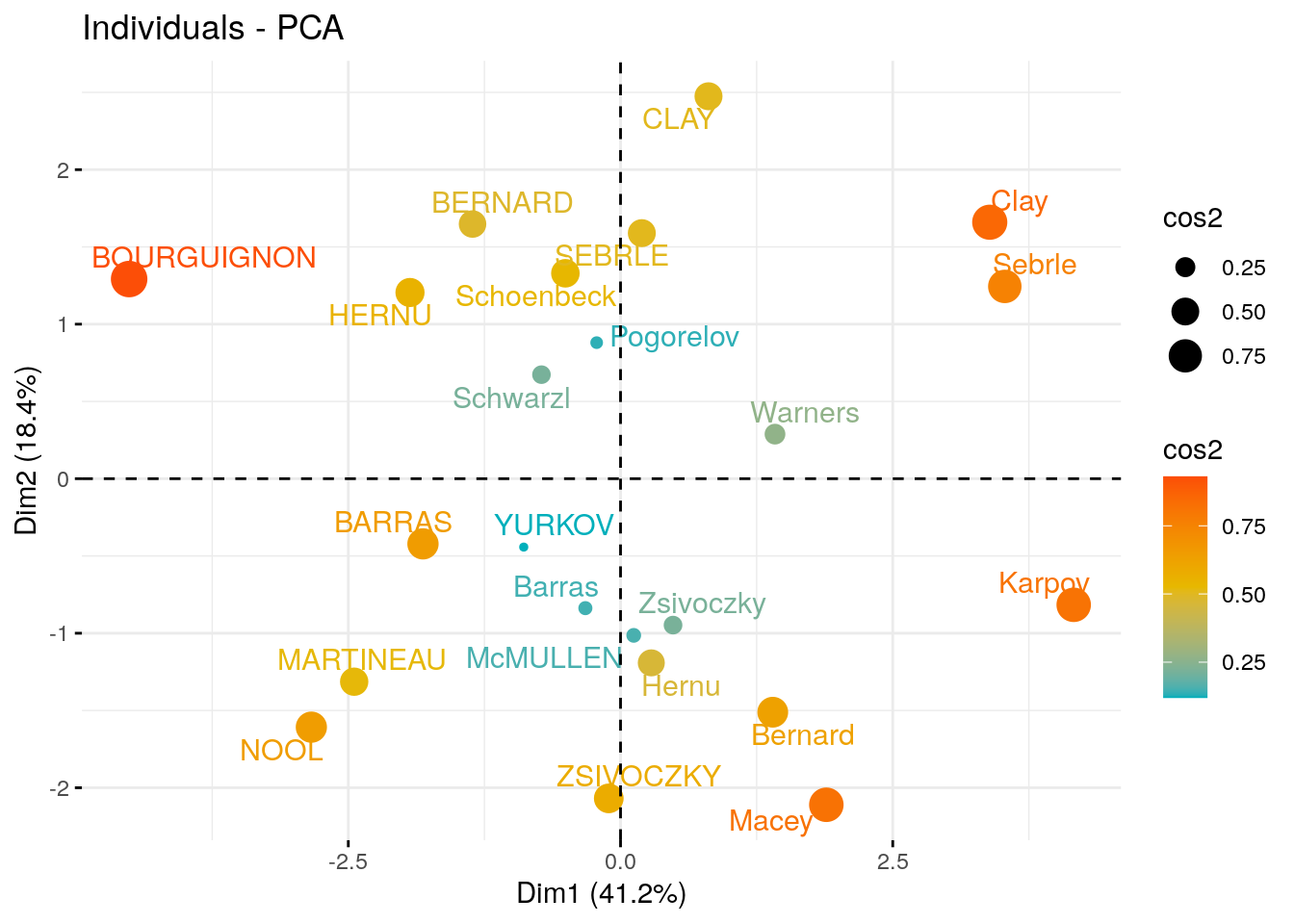
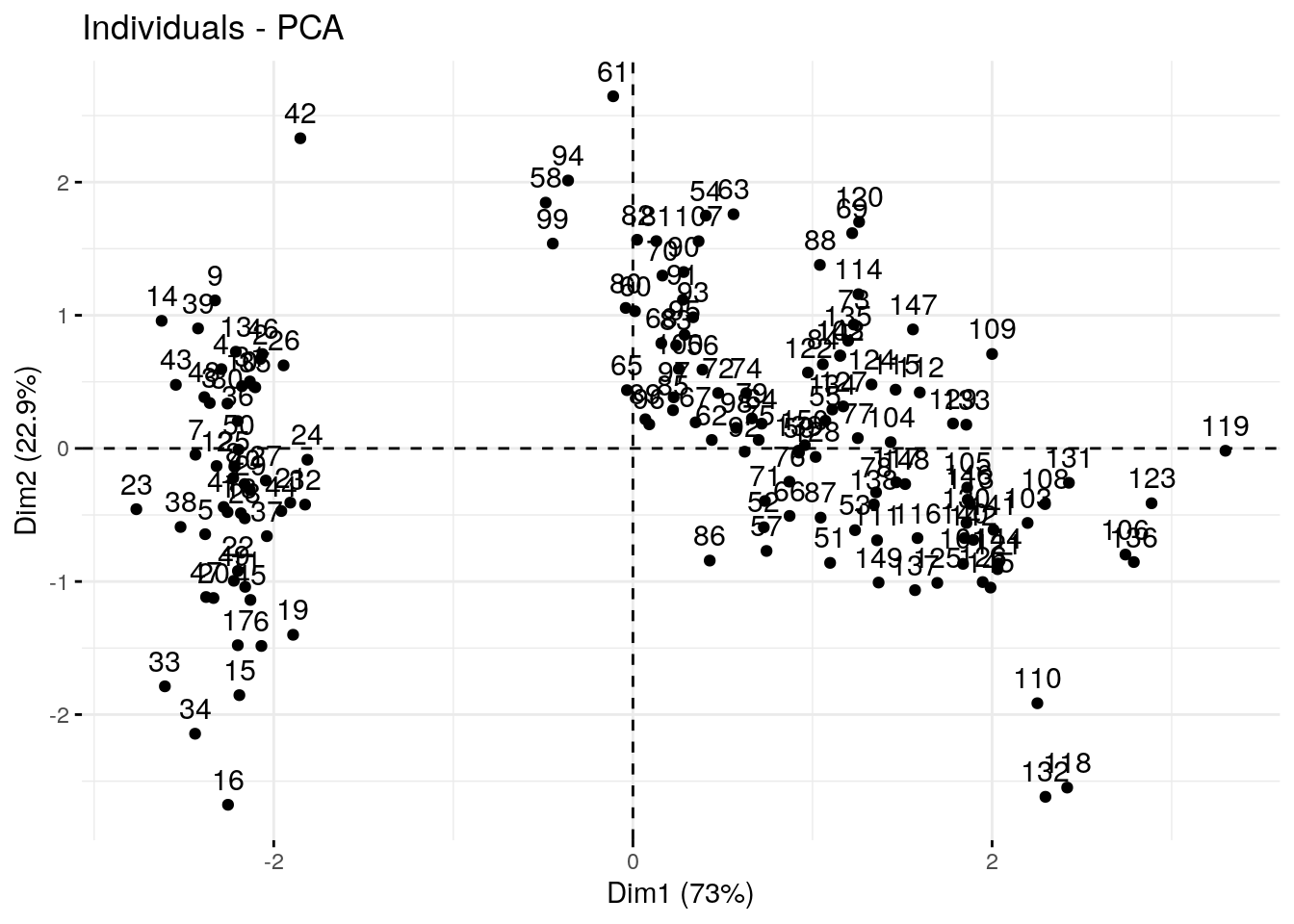
ind <-get_pca_ind(res.pca)ind
Principal Component Analysis Results for individuals
 ===================================================
  Name       Description
1 "$coord"   "Coordinates for the individuals"
2 "$cos2"    "Cos2 for the individuals"
3 "$contrib" "contributions of the individuals"
fviz_pca_ind(res.pca, col.ind ="cos2", gradient.cols =c("#00AFBB", "#E7B800", "#FC4E07"),repel =TRUE# Avoid text overlapping (slow if many points) )
fviz_pca_ind(res.pca, pointsize ="cos2", pointshape =21, fill ="#E7B800",repel =TRUE# Avoid text overlapping (slow if many points) )
fviz_pca_ind(res.pca, col.ind ="cos2", pointsize ="cos2",gradient.cols =c("#00AFBB", "#E7B800", "#FC4E07"),repel =TRUE# Avoid text overlapping (slow if many points) )
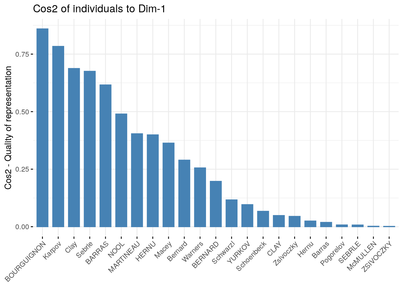
fviz_cos2(res.pca, choice ="ind")
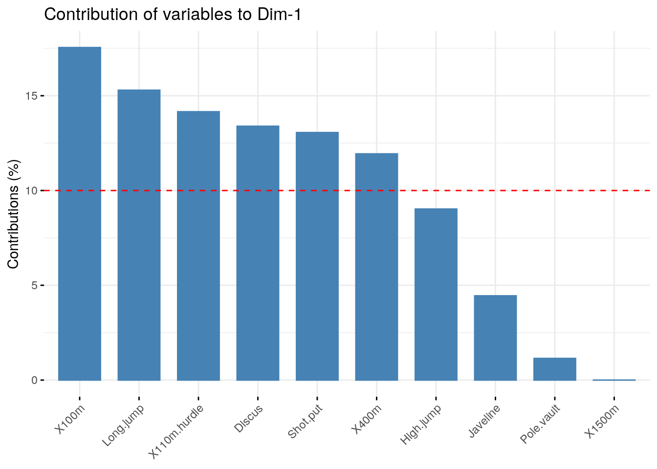
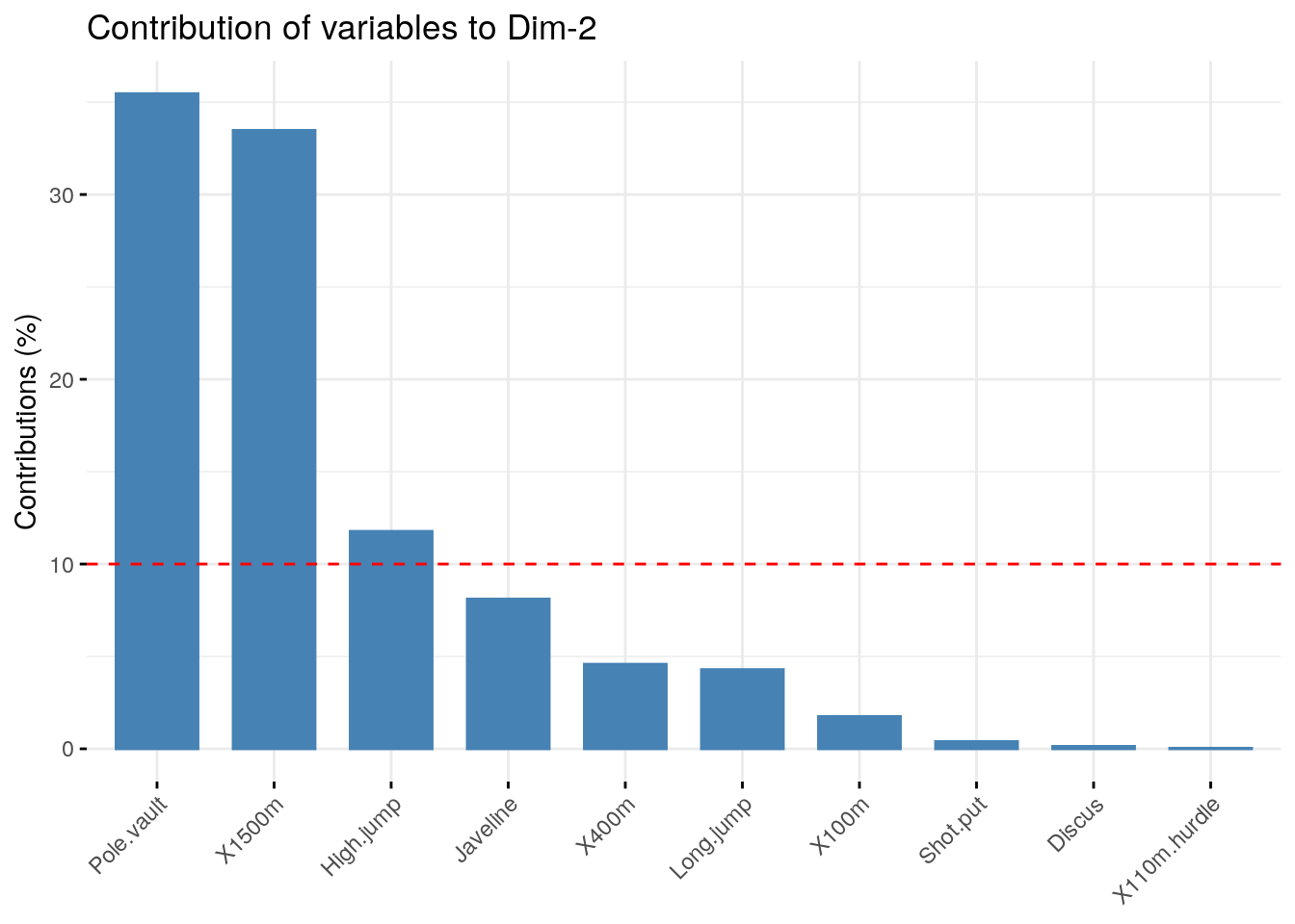
# Total contribution on PC1 and PC2fviz_contrib(res.pca, choice ="ind", axes =1:2)
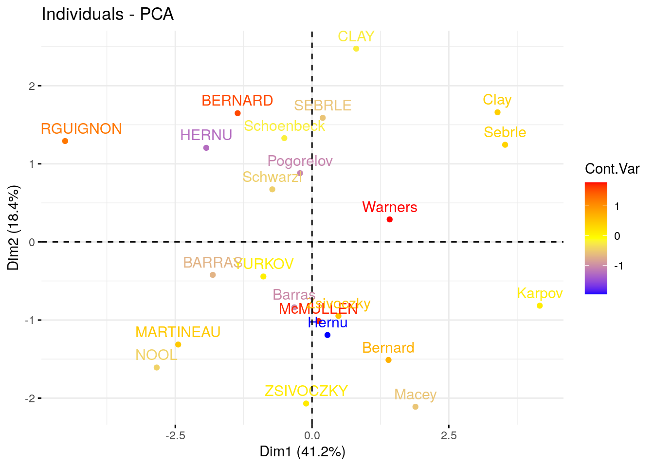
# Create a random continuous variable of length 23,# Same length as the number of active individuals in the PCAset.seed(123)my.cont.var <-rnorm(23)# Color individuals by the continuous variablefviz_pca_ind(res.pca, col.ind = my.cont.var,gradient.cols =c("blue", "yellow", "red"),legend.title ="Cont.Var")
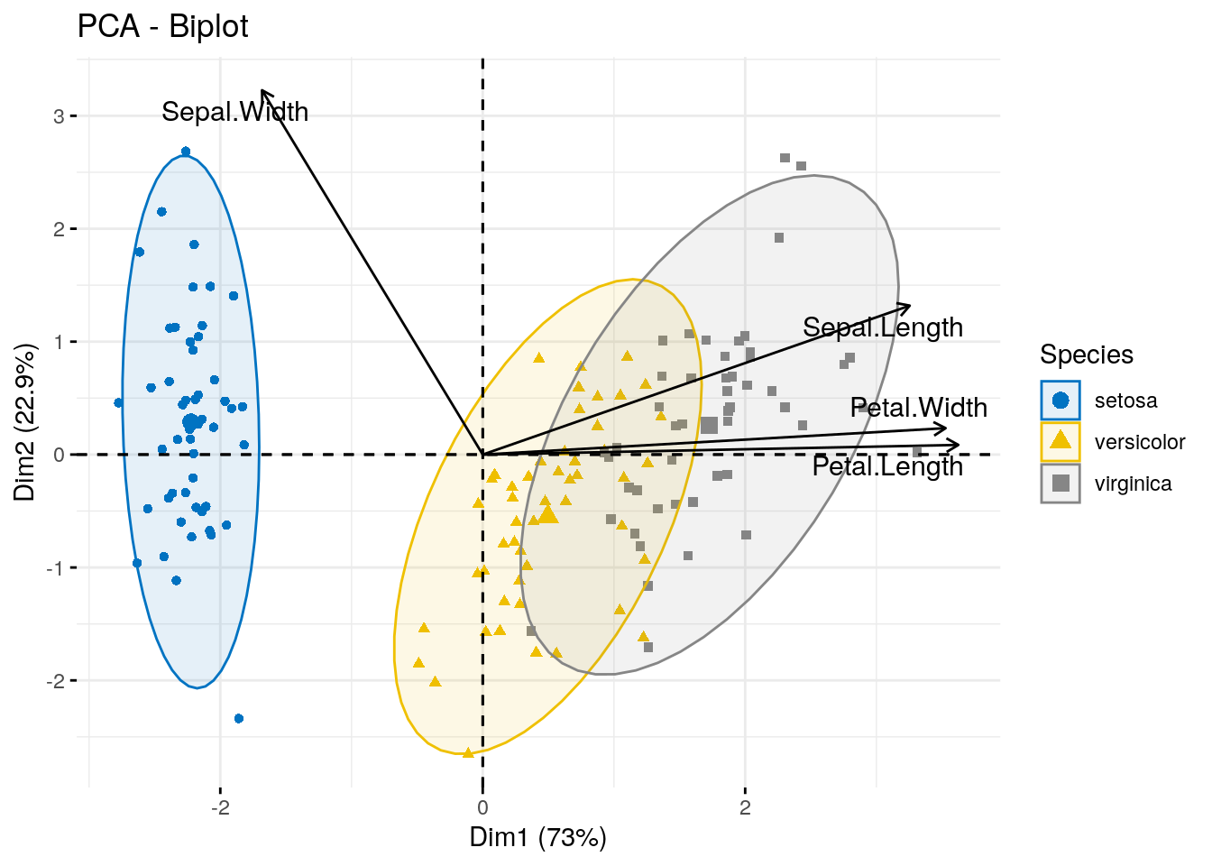
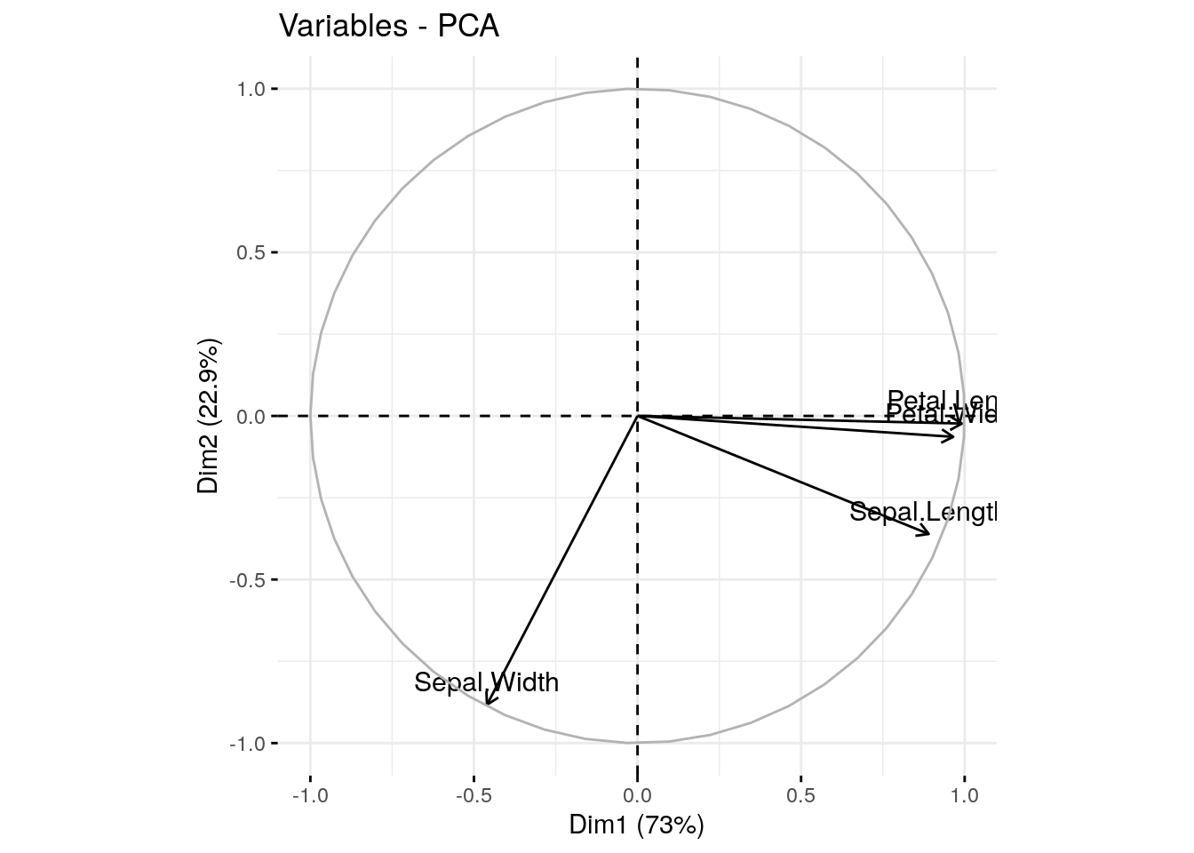
head(iris, 3)
Sepal.Length
Sepal.Width
Petal.Length
Petal.Width
Species
5.1
3.5
1.4
0.2
setosa
4.9
3.0
1.4
0.2
setosa
4.7
3.2
1.3
0.2
setosa
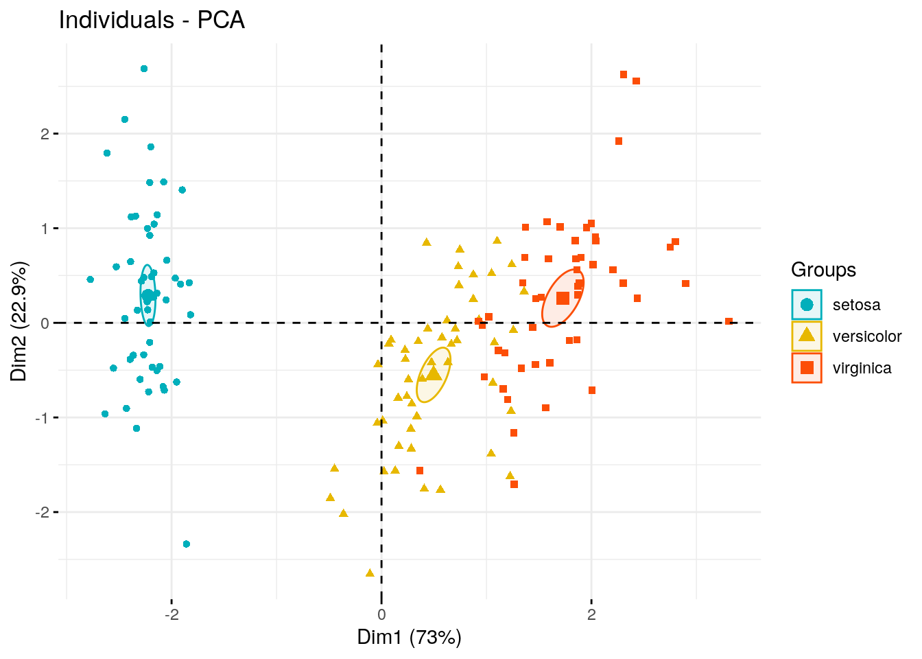
# The variable Species (index = 5) is removed# before PCA analysisiris.pca <-PCA(iris[,-5], graph =FALSE)
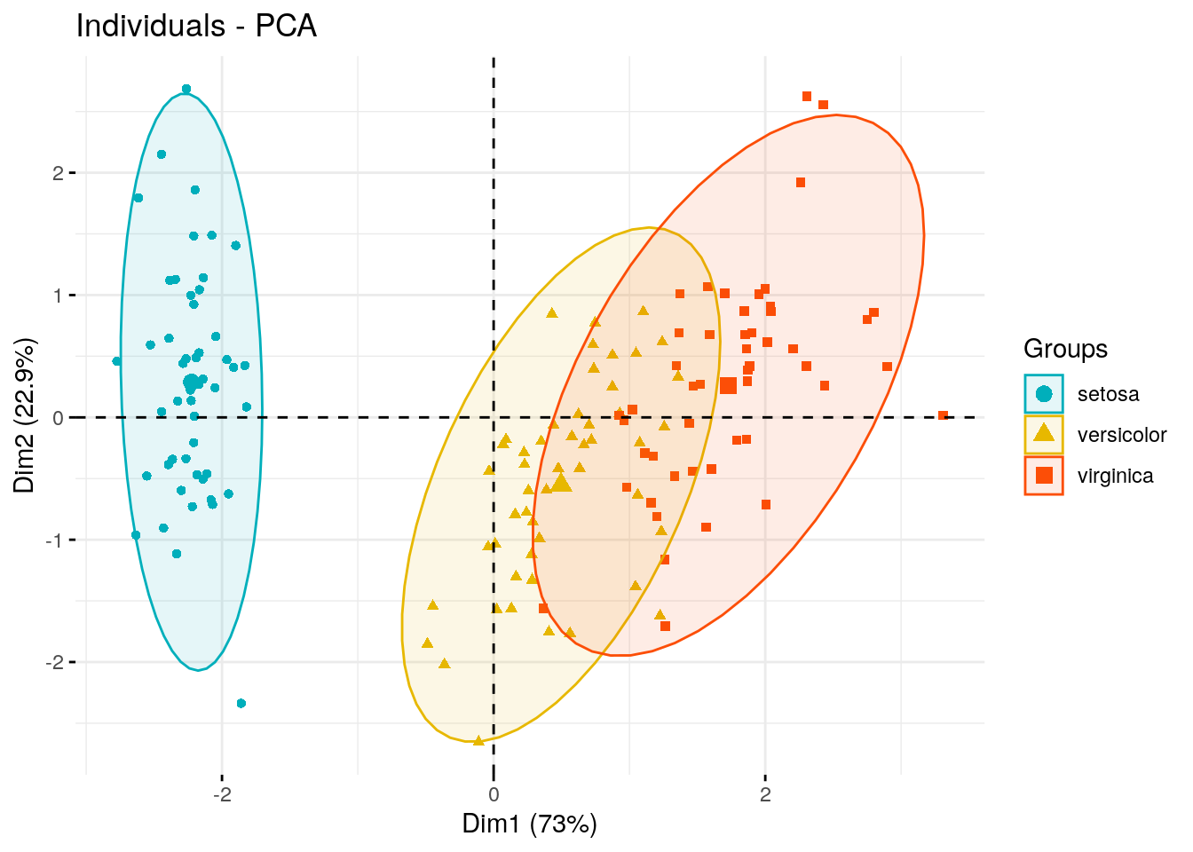
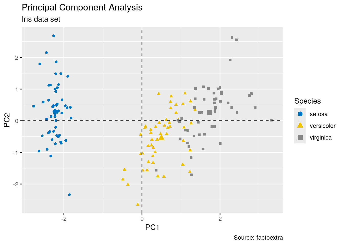
fviz_pca_ind(iris.pca,geom.ind ="point", # show points only (nbut not "text")col.ind = iris$Species, # color by groupspalette =c("#00AFBB", "#E7B800", "#FC4E07"),addEllipses =TRUE, # Concentration ellipseslegend.title ="Groups" )
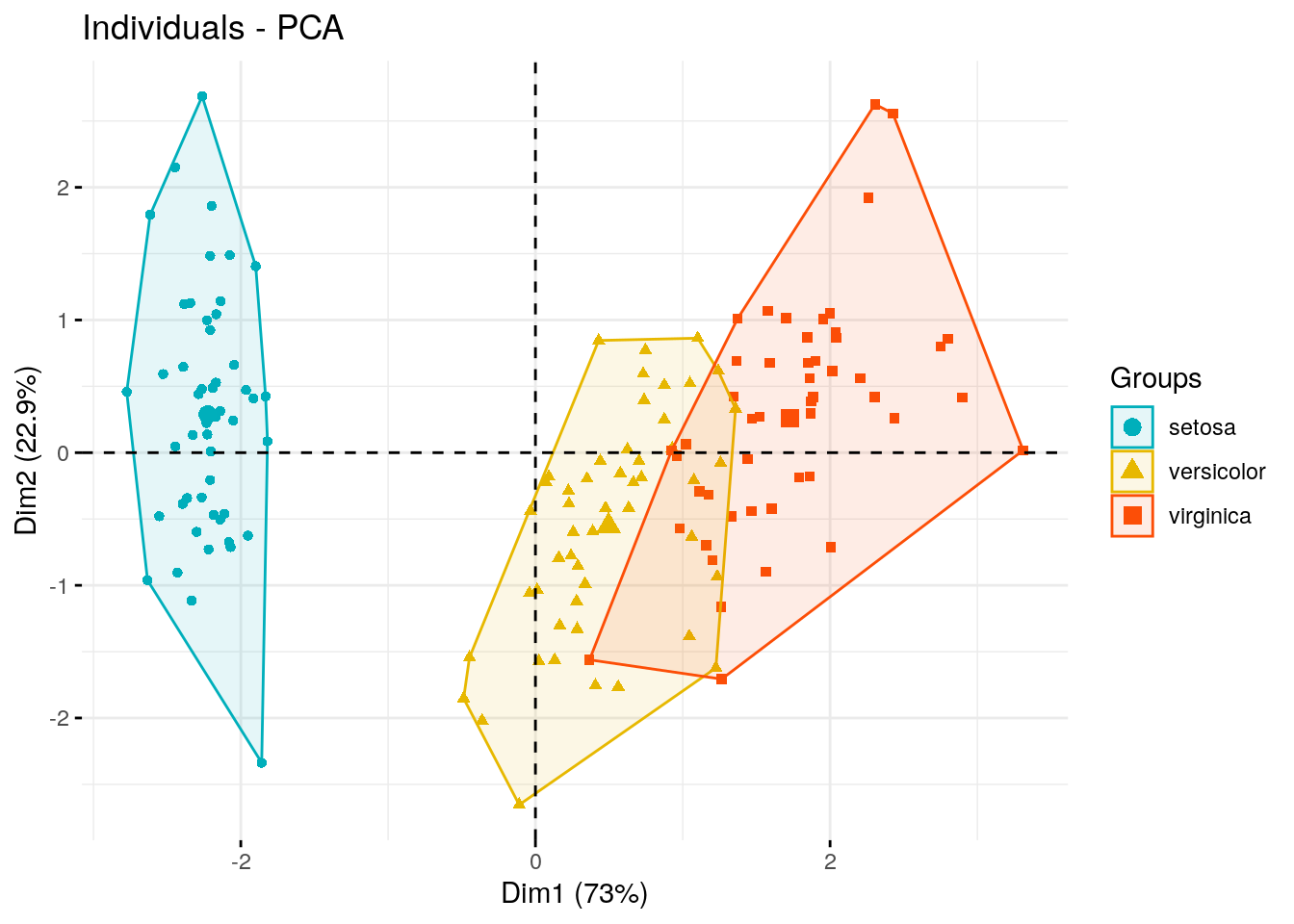
# Convex hullfviz_pca_ind(iris.pca, geom.ind ="point",col.ind = iris$Species, # color by groupspalette =c("#00AFBB", "#E7B800", "#FC4E07"),addEllipses =TRUE, ellipse.type ="convex",legend.title ="Groups" )
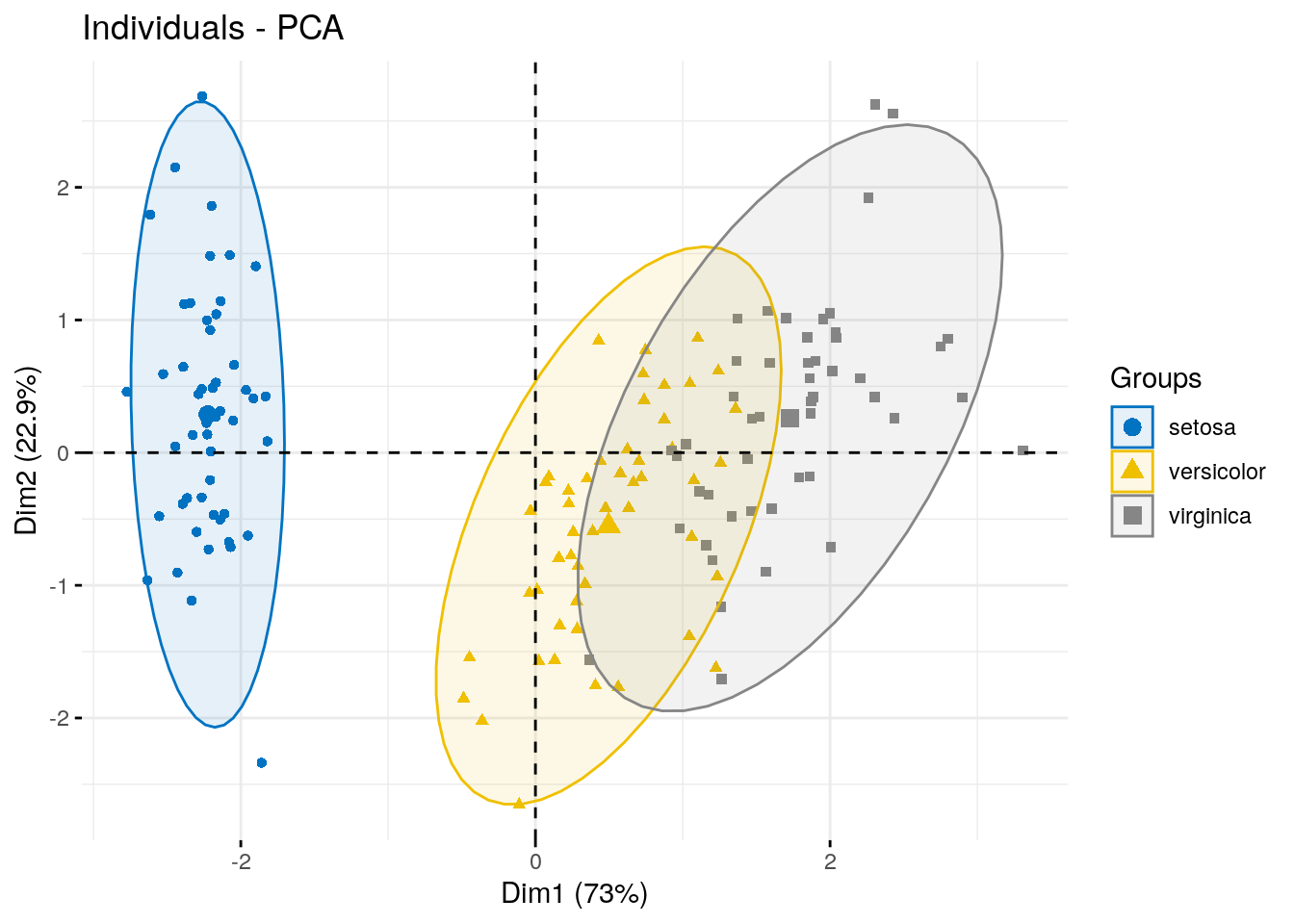
fviz_pca_ind(iris.pca,geom.ind ="point", # show points only (but not "text")group.ind = iris$Species, # color by groupslegend.title ="Groups",mean.point =FALSE)
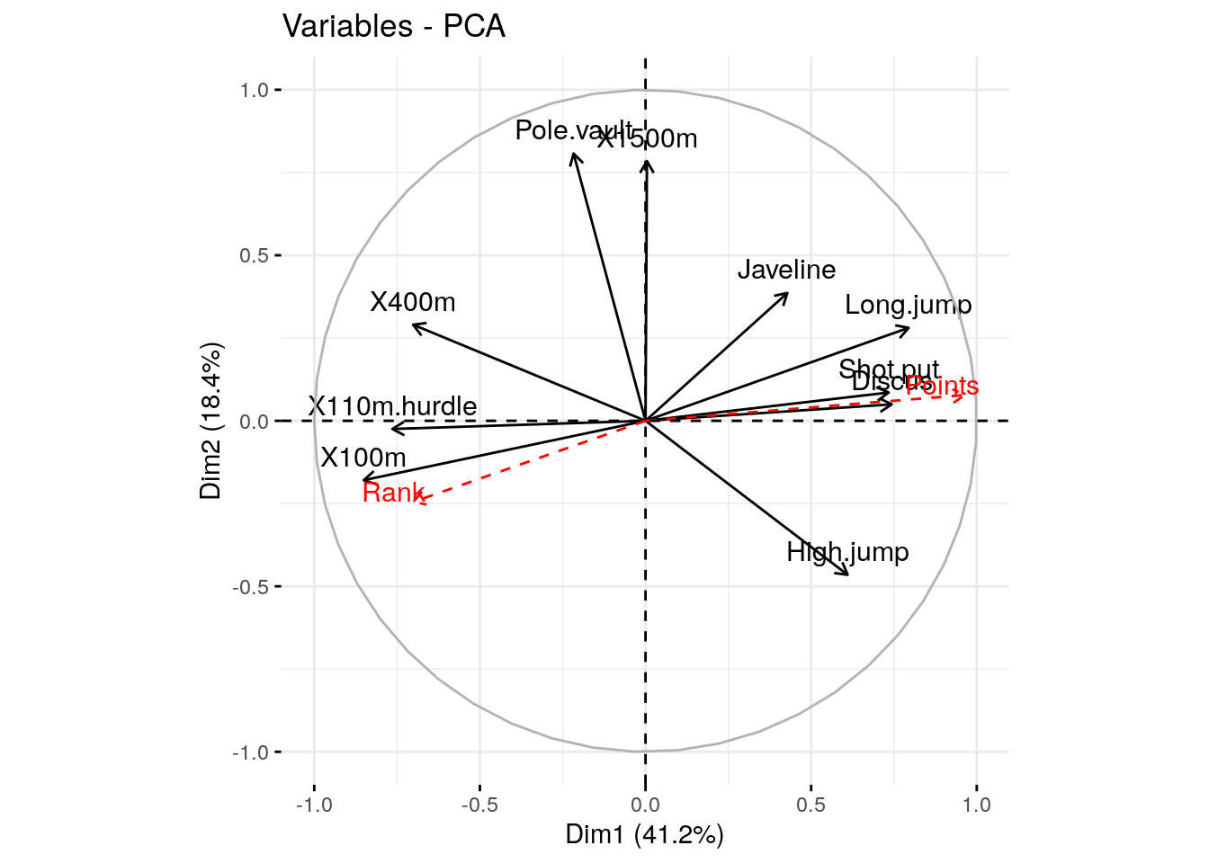
# Plot of active variablesp <-fviz_pca_var(res.pca, invisible ="quanti.sup")# Add supplementary active variablesfviz_add(p, res.pca$quanti.sup$coord, geom =c("arrow", "text"), color ="red")
# top 5 contributing individuals and variablefviz_pca_biplot(res.pca, select.ind =list(contrib =5), select.var =list(contrib =5),ggtheme =theme_minimal())
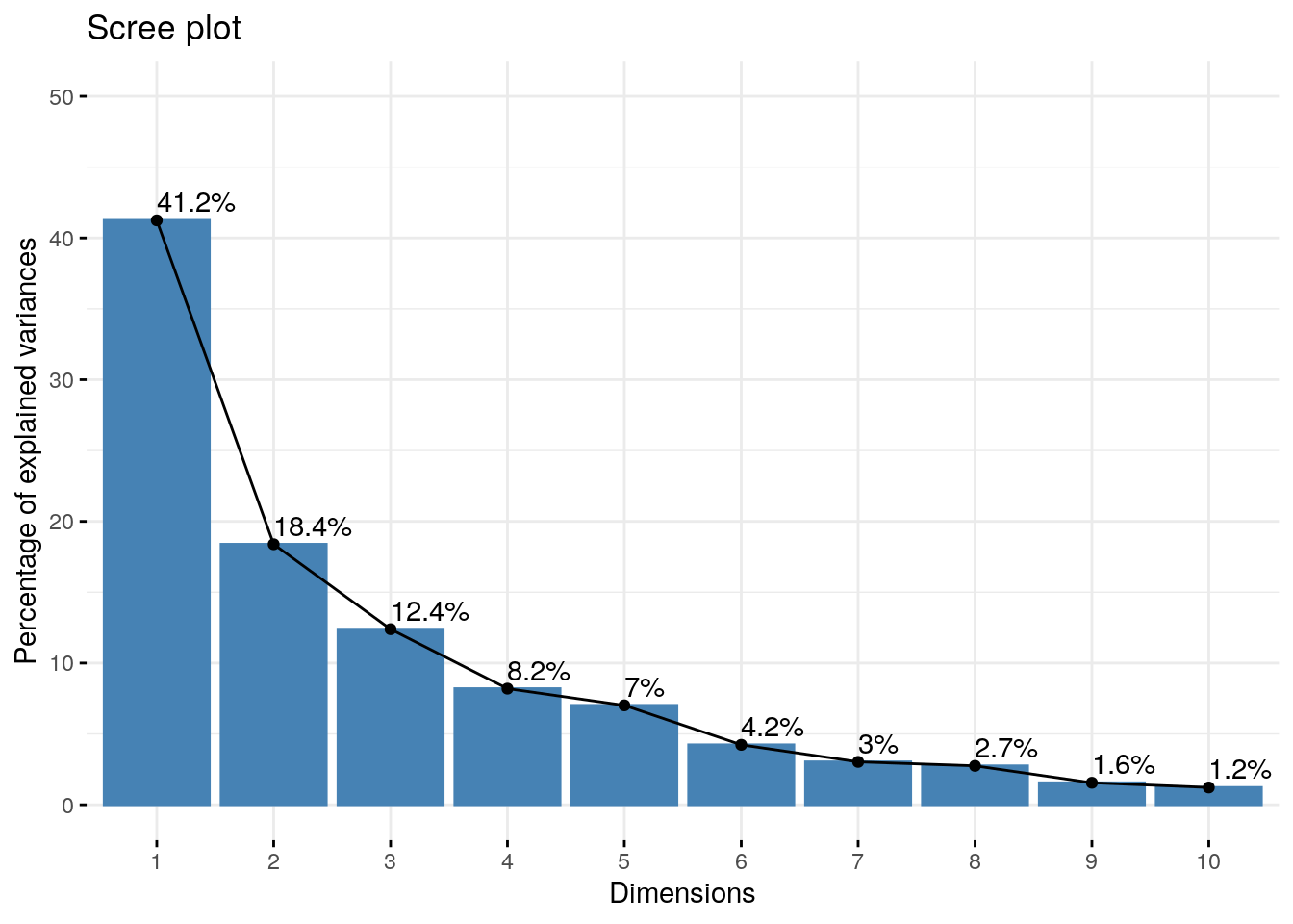
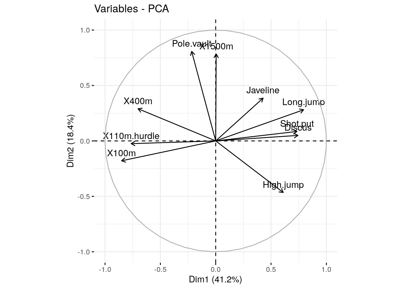
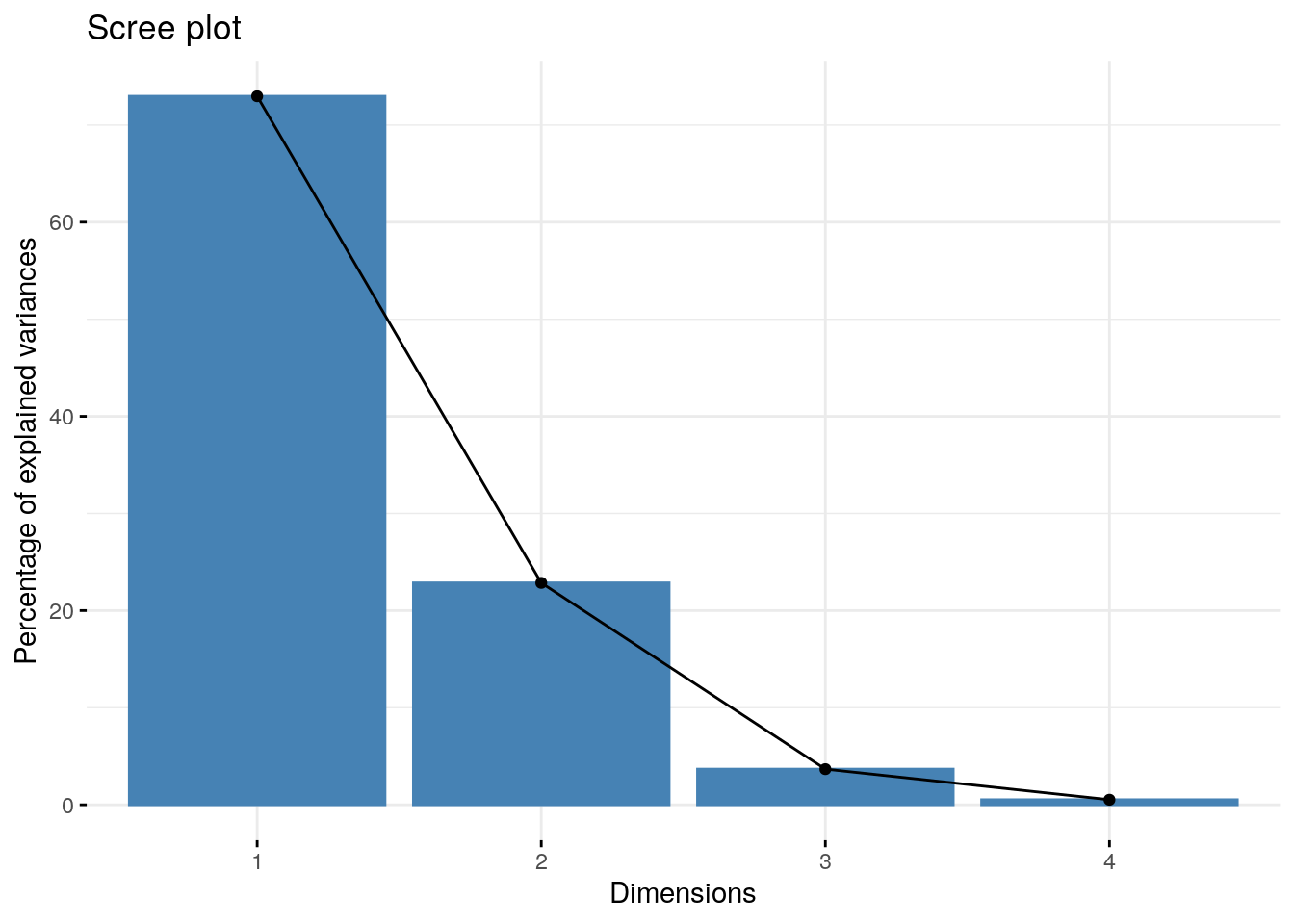
# Scree plotscree.plot <-fviz_eig(res.pca)# Plot of individualsind.plot <-fviz_pca_ind(res.pca)# Plot of variablesvar.plot <-fviz_pca_var(res.pca)pdf("data/PCA.pdf") # Create a new pdf deviceprint(scree.plot)print(ind.plot)print(var.plot)dev.off() # Close the pdf device
png
  2
# Print scree plot to a png filepng("data/pca-scree-plot.png")print(scree.plot)dev.off()
png
  2
# Print individuals plot to a png filepng("data/pca-variables.png")print(var.plot)dev.off()
png
  2
# Print variables plot to a png filepng("data/pca-individuals.png")print(ind.plot)dev.off()
No matter what functions you decide to use, in the list above, the factoextra package can handle the output for creating beautiful plots similar to what we described in the previous sections for FactoMineR: